Inserm Workshop 282 - practical session
Mediation analyses with the ltmle and medoutcon packages
2025-10-13
Chapter 1 Introduction
 of the workshop](images/url.jpg)
Figure 1.1: QR code towards the github repository of the workshop
We will use the following data set, you can download the data and import it in R.
For example, you can create a R project folder for this practical session, add a “data” folder and copy-paste the “df.csv” file in the data folder.
1.1 Data generating system
The data generating mechanism is defined by the following set of structural equations, where:
- baseline confounders are sex (\(L(0)_{sex}\), 0 for women, 1 for men) and low parental education level (\(L(0)_{low.par.edu}\), 0 for no, 1 for yes),
- the exposure of interest is the individual’s educational level (\(A_{edu}\), 0 for high, 1 for low),
- 2 intermediate confounders affected by the exposure: physical activity (\(L(1)_{phys}\), 0 for no, 1 for yes) and occupation (\(L(1)_{occupation}\), 0 for non-manual, 1 for manual),
- the mediator of interest is smoking (\(M_{smoking}\), 0 for no, 1 for yes),
- the outcome \(Y\) can be death (0 for no, 1 for yes) or a continuous functional score (higher values correspond to higher function).
\[ \begin{array}{lll} L(0)_{sex} &=& f\left(U_{sex}\right) \\ L(0)_{low.par.edu} &=& f\left(L(0)_{sex}, U_{low.par.edu}\right) \\ A_{edu} &=& f\left(L(0)_{sex}, L(0)_{low.par.edu}, U_{edu}\right) \\ L(1)_{phys} &=& f\left(L(0)_{sex}, L(0)_{low.par.edu}, A_{edu}, U_{L(1)_{phys}}\right) \\ L(1)_{occupation} &=& f\left(L(0)_{sex}, L(0)_{low.par.edu}, A_{edu}, L(1)_{phys}, U_{L(1)_{occupation}}\right) \\ M_{smoking} &=& f\left(L(0)_{sex}, L(0)_{low.par.edu}, A_{edu}, L(1)_{phys}, L(1)_{occupation}, U_{M_{smoking}}\right) \\ Y &=& f\left(L(0)_{sex}, L(0)_{low.par.edu}, A_{edu}, L(1)_{phys}, L(1)_{occupation}, M_{smoking}, U_Y \right) \\ \end{array}\]
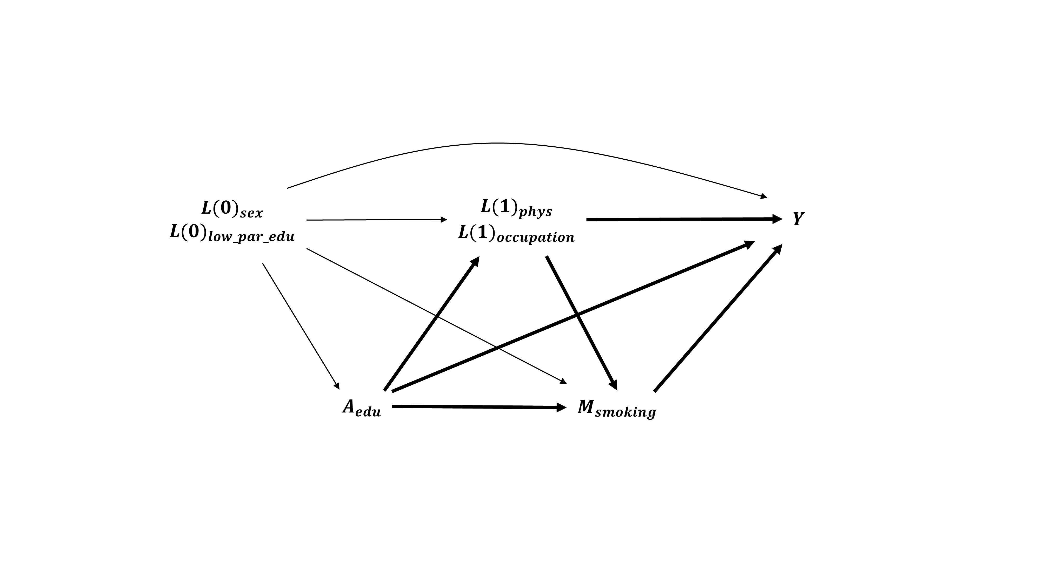
Figure 1.2: Causal model 1
Data were simulated using simple logistic and linear models.
Note that an “exposure - mediator” interaction term is included in the equations to simulate the binary and quantitative outcomes. This will have to be considered during the estimations (in case of exposure-mediator interaction, the results will depend on the choice of estimands: pure or total indirect and direct effects).
## The following function can be used to simulate data.frames and estimate
## the "true" Average total effect and controlled direct effects
GenerateData.CDE <- function(N,
                             inter = rep(1, N), # presence of A*M interaction
                             psi = FALSE) { # FALSE = simulate data.fame only
  ### rexpit function
  rexpit <- function (x) rbinom(length(x), 1, plogis(x))

  ### baseline confounders L0
  sex <- rbinom(N, size = 1, prob = 0.45) # 0 = women; 1 = men
  low_par_edu <- rexpit(qlogis(0.7) + log(1.5) * sex) # low parent education

  ### exposure A: low educational level = 1
  edu <- rexpit(qlogis(0.5) + log(0.8) * sex  + log(2) * low_par_edu)
  edu0 <- rep(0, N)
  edu1 <- rep(1, N)

  ### intermediate counfounders L1
  # physical activity: 1 = yes ; 0 = no
  phys <- rexpit(qlogis(0.6) + log(1.5) * sex  + log(0.8) * low_par_edu +
                   log(0.7) * edu)
  phys0 <- rexpit(qlogis(0.6) + log(1.5) * sex  + log(0.8) * low_par_edu +
                    log(0.7) * edu0)
  phys1 <- rexpit(qlogis(0.6) + log(1.5) * sex  + log(0.8) * low_par_edu +
                    log(0.7) * edu1)

  # occupation: 1 = manual; 0 = non-manual
  occupation <- rexpit(qlogis(0.5) + log(1.3) * sex  + log(1.2) * low_par_edu +
                   log(2.5) * edu + log(2) * phys)
  occupation0 <- rexpit(qlogis(0.5) + log(1.3) * sex  + log(1.2) * low_par_edu +
                          log(2.5) * edu0 + log(2) * phys0)
  occupation1 <- rexpit(qlogis(0.5) + log(1.3) * sex  + log(1.2) * low_par_edu +
                          log(2.5) * edu1 + log(2) * phys1)

  ### mediator
  smoking <- rexpit(qlogis(0.3) + log(1.8) * sex  + log(1.5) * low_par_edu +
                      log(2) * edu + log(0.7) * phys + log(1.8) * occupation)
  smoking0 <- rep(0, N)
  smoking1 <- rep(1, N)
  smoking_tot0 <- rexpit(qlogis(0.3) + log(1.8) * sex  + log(1.5) * low_par_edu +
                           log(2) * edu0 + log(0.7) * phys0 + log(1.8) * occupation0)
  smoking_tot1 <- rexpit(qlogis(0.3) + log(1.8) * sex  + log(1.5) * low_par_edu +
                           log(2) * edu1 + log(0.7) * phys1 + log(1.8) * occupation1)


  ### outcomes
  death <- rexpit(qlogis(0.05) + log(1.5) * sex  + log(1.6) * low_par_edu +
                    log(1.7) * edu + log(0.8) * phys + log(1.5) * occupation +
                    log(2.5) * smoking + log(1.5) * edu * smoking * inter)
  death00 <- rexpit(qlogis(0.05) + log(1.5) * sex  + log(1.6) * low_par_edu +
                      log(1.7) * edu0 + log(0.8) * phys0 + log(1.5) * occupation0 +
                      log(2.5) * smoking0 + log(1.5) * edu0 * smoking0 * inter)
  death01 <- rexpit(qlogis(0.05) + log(1.5) * sex  + log(1.6) * low_par_edu +
                      log(1.7) * edu0 + log(0.8) * phys0 + log(1.5) * occupation0 +
                      log(2.5) * smoking1 + log(1.5) * edu0 * smoking1 * inter)
  death10 <- rexpit(qlogis(0.05) + log(1.5) * sex  + log(1.6) * low_par_edu +
                      log(1.7) * edu1 + log(0.8) * phys1 + log(1.5) * occupation1 +
                      log(2.5) * smoking0 + log(1.5) * edu1 * smoking0 * inter)
  death11 <- rexpit(qlogis(0.05) + log(1.5) * sex  + log(1.6) * low_par_edu +
                      log(1.7) * edu1 + log(0.8) * phys1 + log(1.5) * occupation1 +
                      log(2.5) * smoking1 + log(1.5) * edu1 * smoking1 * inter)
  death_tot0 <- rexpit(qlogis(0.05) + log(1.5) * sex  + log(1.6) * low_par_edu +
                         log(1.7) * edu0 + log(0.8) * phys0 + log(1.5) * occupation0 +
                         log(2.5) * smoking_tot0 + log(1.5) * edu0 * smoking_tot0 * inter)
  death_tot1 <- rexpit(qlogis(0.05) + log(1.5) * sex  + log(1.6) * low_par_edu +
                         log(1.7) * edu1 + log(0.8) * phys1 + log(1.5) * occupation1 +
                         log(2.5) * smoking_tot1 + log(1.5) * edu1 * smoking_tot1 * inter)

  score <- rnorm(N, mean = 50 + 5 * sex  -5 * low_par_edu +
                   -10 * edu + 8 * phys -7 * occupation +
                   -15 * smoking + -8 * edu * smoking * inter,
                 sd = 15)
  score00 <- rnorm(N, mean = 50 + 5 * sex  -5 * low_par_edu +
                     -10 * edu0 + 8 * phys0 -7 * occupation0 +
                     -15 * smoking0 + -8 * edu0 * smoking0 * inter,
                   sd = 15)
  score01 <- rnorm(N, mean = 50 + 5 * sex  -5 * low_par_edu +
                     -10 * edu0 + 8 * phys0 -7 * occupation0 +
                     -15 * smoking1 + -8 * edu0 * smoking1 * inter,
                   sd = 15)
  score10 <- rnorm(N, mean = 50 + 5 * sex  -5 * low_par_edu +
                     -10 * edu1 + 8 * phys1 -7 * occupation1 +
                     -15 * smoking0 + -8 * edu1 * smoking0 * inter,
                   sd = 15)
  score11 <- rnorm(N, mean = 50 + 5 * sex  -5 * low_par_edu +
                     -10 * edu1 + 8 * phys1 -7 * occupation1 +
                     -15 * smoking1 + -8 * edu1 * smoking1 * inter,
                   sd = 15)
  score_tot0 <- rnorm(N, mean = 50 + 5 * sex  -5 * low_par_edu +
                        -10 * edu0 + 8 * phys0 -7 * occupation0 +
                        -15 * smoking_tot0 + -8 * edu0 * smoking_tot0 * inter,
                      sd = 15)
  score_tot1 <- rnorm(N, mean = 50 + 5 * sex  -5 * low_par_edu +
                        -10 * edu1 + 8 * phys1 -7 * occupation1 +
                        -15 * smoking_tot1 + -8 * edu1 * smoking_tot1 * inter,
                      sd = 15)


  if (psi == FALSE) {
    return(data.sim = data.frame(subjid = 1:N,
                                 sex = sex,
                                 low_par_edu = low_par_edu,
                                 edu = edu,
                                 phys = phys,
                                 occupation = occupation,
                                 smoking = smoking,
                                 death = death,
                                 score = score))
  } else {
    return(Psi = list(EY00_death = mean(death00),
                      EY01_death = mean(death01),
                      EY10_death = mean(death10),
                      EY11_death = mean(death11),
                      EY0_death = mean(death_tot0),
                      EY1_death = mean(death_tot1),
                      ATE_death = mean(death_tot1) - mean(death_tot0),
                      CDE0_death = mean(death10) - mean(death00),
                      CDE1_death = mean(death11) - mean(death01),
                      EY00_score = mean(score00),
                      EY01_score = mean(score01),
                      EY10_score = mean(score10),
                      EY11_score = mean(score11),
                      EY0_score = mean(score_tot0),
                      EY1_score = mean(score_tot1),
                      ATE_score = mean(score_tot1) - mean(score_tot0),
                      CDE0_score = mean(score10) - mean(score00),
                      CDE1_score = mean(score11) - mean(score01)))
  }
}


## Simulate the data.frame df
set.seed(1234)
df <- GenerateData.CDE(N = 10000, inter = rep(1, 10000), psi = FALSE)
summary(df)
## subjid sex low_par_edu edu
## Min. : 1 Min. :0.0000 Min. :0.0000 Min. :0.0000
## 1st Qu.: 2501 1st Qu.:0.0000 1st Qu.:0.0000 1st Qu.:0.0000
## Median : 5000 Median :0.0000 Median :1.0000 Median :1.0000
## Mean : 5000 Mean :0.4488 Mean :0.7329 Mean :0.5953
## 3rd Qu.: 7500 3rd Qu.:1.0000 3rd Qu.:1.0000 3rd Qu.:1.0000
## Max. :10000 Max. :1.0000 Max. :1.0000 Max. :1.0000
## phys occupation smoking death
## Min. :0.0000 Min. :0.000 Min. :0.0000 Min. :0.0000
## 1st Qu.:0.0000 1st Qu.:0.000 1st Qu.:0.0000 1st Qu.:0.0000
## Median :1.0000 Median :1.000 Median :1.0000 Median :0.0000
## Mean :0.5579 Mean :0.744 Mean :0.5842 Mean :0.2561
## 3rd Qu.:1.0000 3rd Qu.:1.000 3rd Qu.:1.0000 3rd Qu.:1.0000
## Max. :1.0000 Max. :1.000 Max. :1.0000 Max. :1.0000
## score
## Min. :-49.40
## 1st Qu.: 15.18
## Median : 30.37
## Mean : 30.48
## 3rd Qu.: 45.67
## Max. : 97.00## Calculate the "true" estimands for:
## - the Average total effect: ATE = E(Y_0) - E(Y_1)
## - the controlled direct effect CDE(M=m), setting the mediator to M=m
## CDE(M=0) = E(Y_10) - E(Y_00)
## CDE(M=1) = E(Y_11) - E(Y_01)
set.seed(1234)
true <- GenerateData.CDE(N = 10000, inter = rep(1, 1e6), psi = TRUE) # CHANGE N TO 1e6 ++++++++++
true## $EY00_death
## [1] 0.096781
##
## $EY01_death
## [1] 0.209633
##
## $EY10_death
## [1] 0.163479
##
## $EY11_death
## [1] 0.416236
##
## $EY0_death
## [1] 0.153527
##
## $EY1_death
## [1] 0.332711
##
## $ATE_death
## [1] 0.179184
##
## $CDE0_death
## [1] 0.066698
##
## $CDE1_death
## [1] 0.206603
##
## $EY00_score
## [1] 48.78223
##
## $EY01_score
## [1] 33.57381
##
## $EY10_score
## [1] 36.85815
##
## $EY11_score
## [1] 13.95586
##
## $EY0_score
## [1] 41.77577
##
## $EY1_score
## [1] 21.84661
##
## $ATE_score
## [1] -19.92916
##
## $CDE0_score
## [1] -11.92408
##
## $CDE1_score
## [1] -19.61794