Chapter 6 G-computation
If we make the assumption that the intermediate confounder \(L(1)\) of the \(M-Y\) relationship is affected by the exposure \(A\) (Causal model 2, Figure 3.2), it is necessary to use other methods than traditional regressions models. To illustrate g-computation estimators, we will use the df2_int.csv data set, which was generated from a system corresponding to this assumption. Moreover, we will assume that there is an \(A \star M\) interaction effect on the outcome.
G-computation can be used for the estimation of the total effect and two-way decomposition (CDE, marginal and conditional randomized direct and indirect effects). Analogs of the 3-way and 4-way decompositions are also given by the CMAverse package.
6.1 Estimation of the Average Total Effect (ATE)
The following steps describe the implementation of the g-computation estimator of the average total effect \(\text{ATE} = \mathbb{E}(Y_{A=1}) - \mathbb{E}(Y_{A=0})\):
Fit a logistic or a linear regression to estimate \(\overline{Q} = \mathbb{E}(Y \mid A, L(0))\)
Use this estimate to predict an outcome for each subject \(\hat{\overline{Q}}(A=0)_i\) and \(\hat{\overline{Q}}(A=1)_i\), by evaluating the regression fit \(\overline{Q}\) at \(A=0\) and \(A=1\) respectively
Plug the predicted outcomes in the g-formula and use the sample mean to estimate \(\Psi_{ATE}\) \[\begin{equation} \hat{\Psi}^{\text{ATE}}_{\text{gcomp}} = \frac{1}{n} \sum_{i=1}^n \left[ \hat{\overline{Q}}(A=1)_i - \hat{\overline{Q}}(A=0)_i \right] \end{equation}\]
For continuous outcomes, \(\overline{Q}(A=a)\) functions can be estimated using linear regressions. For binary outcomes, they can be estimated using logistic regressions.
## 0. Import data
rm(list=ls())
df2_int <- read.csv(file = "./data/df2_int.csv")

## 1. Estimate Qbar
Q.tot.death <- glm(Y_death ~ A0_PM2.5 + L0_male + L0_soc_env,
                   family = "binomial", data = df2_int)
Q.tot.qol <- glm(Y_qol ~ A0_PM2.5 + L0_male + L0_soc_env,
                 family = "gaussian", data = df2_int)

## 2. Predict an outcome for each subject, setting A=0 and A=1
# prepare data sets used to predict the outcome under the counterfactual
# scenarios setting A=0 and A=1
data.A1 <- data.A0 <- df2_int
data.A1$A0_PM2.5 <- 1
data.A0$A0_PM2.5 <- 0

# predict values
Y1.death.pred <- predict(Q.tot.death, newdata = data.A1, type = "response")
Y0.death.pred <- predict(Q.tot.death, newdata = data.A0, type = "response")

Y1.qol.pred <- predict(Q.tot.qol, newdata = data.A1, type = "response")
Y0.qol.pred <- predict(Q.tot.qol, newdata = data.A0, type = "response")

## 3. Plug the predicted outcome in the gformula and use the sample mean
##    to estimate the ATE
ATE.death.gcomp <- mean(Y1.death.pred - Y0.death.pred)
ATE.death.gcomp
# [1] 0.08270821

ATE.qol.gcomp <- mean(Y1.qol.pred - Y0.qol.pred)
ATE.qol.gcomp
# [1] -8.360691
A 95% confidence interval can be estimated applying a bootstrap procedure. An example is given in the following code.
set.seed(1234)
B <- 1000
bootstrap.estimates <- data.frame(matrix(NA, nrow = B, ncol = 2))
colnames(bootstrap.estimates) <- c("boot.death.est", "boot.qol.est")
for (b in 1:B){
  # sample the indices 1 to n with replacement
  bootIndices <- sample(1:nrow(df2_int), replace=T)
  bootData <- df2_int[bootIndices,]

  if (round(b/100, 0) == b/100 ) print(paste0("bootstrap number ",b))

  Q.tot.death <- glm(Y_death ~ A0_PM2.5 + L0_male + L0_soc_env,
                     family = "binomial", data = bootData)
  Q.tot.qol <- glm(Y_qol ~ A0_PM2.5 + L0_male + L0_soc_env,
                   family = "gaussian", data = bootData)

  boot.A.1 <- boot.A.0 <- bootData
  boot.A.1$A0_PM2.5 <- 1
  boot.A.0$A0_PM2.5 <- 0

  Y1.death.boot <- predict(Q.tot.death, newdata = boot.A.1, type = "response")
  Y0.death.boot <- predict(Q.tot.death, newdata = boot.A.0, type = "response")

  Y1.qol.boot <- predict(Q.tot.qol, newdata = boot.A.1, type = "response")
  Y0.qol.boot <- predict(Q.tot.qol, newdata = boot.A.0, type = "response")

  bootstrap.estimates[b,"boot.death.est"] <- mean(Y1.death.boot - Y0.death.boot)
  bootstrap.estimates[b,"boot.qol.est"] <- mean(Y1.qol.boot - Y0.qol.boot)
}

IC95.ATE.death <- c(ATE.death.gcomp -
                      qnorm(0.975) * sd(bootstrap.estimates[,"boot.death.est"]),
                    ATE.death.gcomp +
                      qnorm(0.975) * sd(bootstrap.estimates[,"boot.death.est"]))
IC95.ATE.death
# [1] 0.05612907 0.10928734

IC95.ATE.qol <- c(ATE.qol.gcomp -
                    qnorm(0.975) * sd(bootstrap.estimates[,"boot.qol.est"]),
                  ATE.qol.gcomp +
                    qnorm(0.975) * sd(bootstrap.estimates[,"boot.qol.est"]))
IC95.ATE.qol
# [1] -9.157856 -7.563526
6.2 Estimation of Controlled Direct Effects (CDE)
The controlled direct effect \(\Psi^{\text{CDE}_m} = \mathbb{E}(Y_{A=1,M=m}) - \mathbb{E}(Y_{A=0,M=m})\) is the difference between the mean outcome had the whole population been exposed to high levels of \(\text{PM}_{2.5}\) (setting \(A=1\)), compared to the mean outcome had the whole population been unexposed (setting \(A=0\)), while keeping the mediator (type-2 diabetes) equal to a constant given value (\(M=m\)) in both scenarios.
The g-formula for a CDE (\(\mathbb{E}(Y_{A=a^\prime,M=m})\)) is more complex than for the average total effect, and the simple substitution approach described previously is less convenient to apply:
\(\mathbb{E}(Y_{A=a^\prime,M=m}) = \sum_{l(0),l(1)} \left[ \mathbb{E}\left(Y \mid m, l(1), a^\prime, l(0) \right) \times P\left( L(1)=l(1) | a^\prime,l(0) \right) \right] \times P\left( L(0)=l(0) \right)\)
In our simple example with a binary exposure \(A\), a binary mediator \(M\) and a binary intermediate confounder \(L(1)\), it is still possible to apply the substitution approach (corresponding to a non-parametric g-computation estimation) by estimating the following components of the g-formula:
- \(\overline{Q}_Y(A,L(1),M)=\mathbb{E}\left(Y \mid L(0), A,L(1), M \right)\),
- and \(\overline{Q}_{L(1)}(A)=P\left(L(1)=1) \mid A, l(0)\right)\)
We can then generate predicted outcomes from these 3 models for each subject in the data set, and obtain a non-parametric maximum likelihood estimator (NPMLE) of the CDE using the empirical mean: \[\scriptsize \begin{array}{r l} \Psi^{\text{CDE}_m}_{\text{NPMLE}} = \frac{1}{n}\sum & \left[\hat{\overline{Q}}_Y(A=1,L(1)=1,M=m) \times \hat{\overline{Q}}_{L(1)}(A=1) + \hat{\overline{Q}}_Y(A=1,L(1)=0,M=m) \times (1 - \hat{\overline{Q}}_{L(1)}(A=1))\right]\\ & - \left[\hat{\overline{Q}}_Y(A=0,L(1)=1,M=m) \times \hat{\overline{Q}}_{L(1)}(A=0) + \hat{\overline{Q}}_Y(A=0,L(1)=0,M=m) \times (1 - \hat{\overline{Q}}_{L(1)}(A=0))\right] \end{array}\]
However NPMLE is tedious with high-dimensional intermediate confounders \(L(1)\) or if mediators is repeated over time. In that case, parametric g-computation using a Monte Carlo algorithm, or g-computation by iterative conditional expectation are easier to apply.
Below, we describe three g-computation procedures for the estimation of a CDE:
- parametric g-computation, using Monte Carlo simulation
- g-computation by iterative conditional expectation
- sequential g-estimator
6.2.1 Parametric g-computation
Parametric g-computation by Monte Carlo simulation have been described by Robins (Robins 1986), Taubman et al. (Taubman et al. 2009), or Daniel et al. (Daniel et al. 2013).
Fit a parametric model to estimate the density of the intermediate confounder \(L(1)\) conditional on its parents. If \(L(1)\) is a set of several variables, it is necessary to fit a model for each variable conditional on its parents (where the \(L(1)\) variables are put in an arbitrary order). \[\begin{equation} Q_{L(1)}(A) = P(L(1)=1 \mid L(0),A) \end{equation}\]
Fit a model of the outcome \(Y\) conditional on its parents: \[\begin{equation} \overline{Q}_Y(A,L(1),M) = \mathbb{E}\left(Y \mid L(0),A,L(1),M \right) \end{equation}\]
Simulate individual values of \(L(1)_a\) using the estimated density \(\hat{Q}_{L(1)}(A=a)\) under the counterfactual scenarios setting \(A=0\) or \(A=1\)
Estimate mean values of the outcome under the counterfactual scenarios setting \(A=0\) (or \(A=1\)), \(L(1)=l(1)_{A=0}\) (or \(L(1)=l(1)_{A=1}\)) and \(M=m\), using \(\hat{\overline{Q}}_Y(A=a,L(1)=l(1)_a,M=m)\)
Estimate the controlled direct effect \(\Psi_{\text{CDE}_m}\) by the sample mean: \[\begin{equation} \small \hat{\Psi}^{\text{CDE}_m}_{\text{param.gcomp}} = \frac{1}{n} \sum_{i=1}^n \left[ \hat{\overline{Q}}_Y(A=1,L(1)=l(1)_{A=1},M=m)_i - \hat{\overline{Q}}_Y(A=0,L(1)=l(1)_{A=0},M=m)_i \right] \end{equation}\]
For continuous outcomes, \(\overline{Q}_Y(A,L(1),M)\) functions can be estimated using linear regressions. For binary outcomes, they can be estimated using logistic regressions.
rm(list=ls())
df2_int <- read.csv(file = "data/df2_int.csv")

## 1. Fit parametric models to estimate the density of intermediate confounders,
##    conditional on the parents of the intermediate confounders
L1.model <- glm(L1 ~ L0_male + L0_soc_env + A0_PM2.5,
                family = "binomial", data = df2_int)

## 2. Fit parametric models for the outcome conditional on past
Y.death.model <- glm(Y_death ~ L0_male + L0_soc_env + A0_PM2.5 + L1 +
                       M_diabetes + A0_PM2.5:M_diabetes,
                     family = "binomial", data = df2_int)

Y.qol.model <- glm(Y_qol ~ L0_male + L0_soc_env + A0_PM2.5 + L1 +
                     M_diabetes + A0_PM2.5:M_diabetes,
                   family = "gaussian", data = df2_int)

## 3. Simulate individual L1 values under the counterfactual scenarios setting A0=0 or A0=1
set.seed(54321)
data.A0  <- data.A1 <- df2_int
data.A0$A0_PM2.5 <- 0
data.A1$A0_PM2.5 <- 1
p.L1.A0 <- predict(L1.model, newdata = data.A0, type="response")
p.L1.A1 <- predict(L1.model, newdata = data.A1, type="response")
sim.L1.A0 <- rbinom(n = nrow(df2_int), size = 1, prob = p.L1.A0)
sim.L1.A1 <- rbinom(n = nrow(df2_int), size = 1, prob = p.L1.A1)

## 4. Estimate mean outcomes under the counterfactual scenarios setting different
##    levels of exposures for A and M:
##    {A=0, M=0} or {A=1, M=0} or {A=0, M=1} or {A=1, M=1}

data.A0.M0 <- data.A0.M1 <- data.A0
data.A1.M0 <- data.A1.M1 <- data.A1

# L1 variable is replaced by the simulated values in step 3)
data.A0.M0$L1 <- sim.L1.A0
data.A0.M1$L1 <- sim.L1.A0
data.A1.M0$L1 <- sim.L1.A1
data.A1.M1$L1 <- sim.L1.A1

# set M to 0 or 1
data.A0.M0$M_diabetes <- 0
data.A0.M1$M_diabetes <- 1
data.A1.M0$M_diabetes <- 0
data.A1.M1$M_diabetes <- 1

# predict the probability of death
p.death.A0.M0 <- predict(Y.death.model, newdata = data.A0.M0, type = "response")
p.death.A1.M0 <- predict(Y.death.model, newdata = data.A1.M0, type = "response")
p.death.A0.M1 <- predict(Y.death.model, newdata = data.A0.M1, type = "response")
p.death.A1.M1 <- predict(Y.death.model, newdata = data.A1.M1, type = "response")

# predict the mean value of QoL
m.qol.A0.M0 <- predict(Y.qol.model, newdata = data.A0.M0, type = "response")
m.qol.A1.M0 <- predict(Y.qol.model, newdata = data.A1.M0, type = "response")
m.qol.A0.M1 <- predict(Y.qol.model, newdata = data.A0.M1, type = "response")
m.qol.A1.M1 <- predict(Y.qol.model, newdata = data.A1.M1, type = "response")

## 5. Estimate the CDE
# CDE setting M=0
CDE.death.m0.gcomp.param <- mean(p.death.A1.M0) - mean(p.death.A0.M0)
CDE.death.m0.gcomp.param
# [1] 0.06289087

CDE.qol.m0.gcomp.param <- mean(m.qol.A1.M0) - mean(m.qol.A0.M0)
CDE.qol.m0.gcomp.param
# [1] -4.838654

# CDE setting M=1
CDE.death.m1.gcomp.param <- mean(p.death.A1.M1) - mean(p.death.A0.M1)
CDE.death.m1.gcomp.param
# [1] 0.08751016

CDE.qol.m1.gcomp.param <- mean(m.qol.A1.M1) - mean(m.qol.A0.M1)
CDE.qol.m1.gcomp.param
# [1] -10.35059
6.2.2 G-computation by iterative conditional expectation
The following steps describe the implementation of the g-computation estimator by iterative conditional expectation for the component \(\mathbb{E}(Y_{A=a^\prime,M=m})\) used in the definition of CDE \(\Psi^{\text{CDE}_m} = \mathbb{E}(Y_{A=1,M=m}) - \mathbb{E}(Y_{A=0,M=m})\). Interestingly, there is no need to estimate or simulate \(L(1)\) density with this method.
Fit a logistic or a linear regression of the final outcome, conditional on the exposure \(A\), the mediator \(M\) and all the parents of \(Y\) preceding \(M\), to estimate \(\overline{Q}_{Y} = \mathbb{E}(Y \mid L(0),A,L(1),M)\);
Use this estimate to predict an outcome for each subject \(\hat{\overline{Q}}_{Y}(A=a^\prime,M=m)_i\), by evaluating the regression fit \(\overline{Q}_{Y}\) at the chosen value for the exposure \(A=a^\prime\) and the mediator \(M=m\);
Fit a quasibinomial or a linear regression of the predicted values \(\hat{\overline{Q}}_{Y}(M=m)_i\) conditional on the exposure \(A\) and baseline confounders \(L(0)\) to estimate \(\overline{Q}_{L(1)} = \mathbb{E}\left(\hat{\overline{Q}}_{Y}(A=a^\prime,M=m) \middle| L(0),A\right)\);
Use this estimate to predict the outcome \(\hat{\overline{Q}}_{L(1)}(A=a^\prime)_i\) for each subject, by evaluating the regression fit \(\overline{Q}_{L(1)}\) at \(A=a^\prime\);
Use the sample mean to estimate \(\Psi^{\text{CDE}_m}_{\text{gcomp}}\) \[\begin{equation} \hat{\Psi}^{\text{CDE}_m}_{\text{gcomp}} = \frac{1}{n} \sum_{i=1}^n \left[ \hat{\overline{Q}}_{L(1)}(A=1)_i - \hat{\overline{Q}}_{L(1)}(A=0)_i \right] \end{equation}\]
Note that G-computation by iterative expectation is preferable if the set of intermediate confounders \(L(1)\) is high-dimensional as we only need to fit 1 model by counterfactual scenario (for a whole set of \(L(1)\) variables) in the procedure described below, whereas at least 1 model by \(L(1)\) variable and by counterfactual scenario are needed with parametric g-computation.
rm(list=ls())
df2_int <- read.csv(file = "data/df2_int.csv")

## 1) Regress the outcome on L0, A, L1 and M (and the A*M interaction if appropriate)
Y.death.model <- glm(Y_death ~ L0_male + L0_soc_env + A0_PM2.5 + L1 +
                       M_diabetes + A0_PM2.5:M_diabetes,
                     family = "binomial", data = df2_int)
Y.qol.model <- glm(Y_qol ~ L0_male + L0_soc_env + A0_PM2.5 + L1 +
                     M_diabetes + A0_PM2.5:M_diabetes,
                   family = "gaussian", data = df2_int)

# 2) Generate predicted values by evaluating the regression setting the exposure
#    and the mediator at exposure history of interest:
#    {A=1,M=0},{A=0,M=0},{A=1,M=1},{A=0,M=1}
data.Ais0.Mis0 <- data.Ais0.Mis1 <- df2_int
data.Ais1.Mis0 <- data.Ais1.Mis1 <- df2_int

data.Ais0.Mis0$A0_PM2.5 <- 0
data.Ais0.Mis0$M_diabetes <- 0

data.Ais0.Mis1$A0_PM2.5 <- 0
data.Ais0.Mis1$M_diabetes <- 1

data.Ais1.Mis0$A0_PM2.5 <- 1
data.Ais1.Mis0$M_diabetes <- 0

data.Ais1.Mis1$A0_PM2.5 <- 1
data.Ais1.Mis1$M_diabetes <- 1

Q.L2.death.A0M0 <- predict(Y.death.model, newdata = data.Ais0.Mis0, type="response")
Q.L2.death.A0M1 <- predict(Y.death.model, newdata = data.Ais0.Mis1, type="response")
Q.L2.death.A1M0 <- predict(Y.death.model, newdata = data.Ais1.Mis0, type="response")
Q.L2.death.A1M1 <- predict(Y.death.model, newdata = data.Ais1.Mis1, type="response")

Q.L2.qol.A0M0 <- predict(Y.qol.model, newdata = data.Ais0.Mis0, type="response")
Q.L2.qol.A0M1 <- predict(Y.qol.model, newdata = data.Ais0.Mis1, type="response")
Q.L2.qol.A1M0 <- predict(Y.qol.model, newdata = data.Ais1.Mis0, type="response")
Q.L2.qol.A1M1 <- predict(Y.qol.model, newdata = data.Ais1.Mis1, type="response")

## 3) Regress the predicted values conditional on the exposure A
##    and baseline confounders L(0)
L1.death.A0M0.model <- glm(Q.L2.death.A0M0 ~ L0_male + L0_soc_env + A0_PM2.5,
                           family = "quasibinomial", data = df2_int)
L1.death.A0M1.model <- glm(Q.L2.death.A0M1 ~ L0_male + L0_soc_env + A0_PM2.5,
                           family = "quasibinomial", data = df2_int)
L1.death.A1M0.model <- glm(Q.L2.death.A1M0 ~ L0_male + L0_soc_env + A0_PM2.5,
                           family = "quasibinomial", data = df2_int)
L1.death.A1M1.model <- glm(Q.L2.death.A1M1 ~ L0_male + L0_soc_env + A0_PM2.5,
                           family = "quasibinomial", data = df2_int)

L1.qol.A0M0.model <- glm(Q.L2.qol.A0M0 ~ L0_male + L0_soc_env + A0_PM2.5,
                         family = "gaussian", data = df2_int)
L1.qol.A0M1.model <- glm(Q.L2.qol.A0M1 ~ L0_male + L0_soc_env + A0_PM2.5,
                         family = "gaussian", data = df2_int)
L1.qol.A1M0.model <- glm(Q.L2.qol.A1M0 ~ L0_male + L0_soc_env + A0_PM2.5,
                         family = "gaussian", data = df2_int)
L1.qol.A1M1.model <- glm(Q.L2.qol.A1M1 ~ L0_male + L0_soc_env + A0_PM2.5,
                         family = "gaussian", data = df2_int)

## 4) generate predicted values by evaluating the regression at exposure
##    of interest: {A=1} & {A=0}
Q.L1.death.A0M0 <- predict(L1.death.A0M0.model, newdata = data.Ais0.Mis0, type="response")
Q.L1.death.A0M1 <- predict(L1.death.A0M1.model, newdata = data.Ais0.Mis1, type="response")
Q.L1.death.A1M0 <- predict(L1.death.A1M0.model, newdata = data.Ais1.Mis0, type="response")
Q.L1.death.A1M1 <- predict(L1.death.A1M1.model, newdata = data.Ais1.Mis1, type="response")

Q.L1.qol.A0M0 <- predict(L1.qol.A0M0.model, newdata = data.Ais0.Mis0, type="response")
Q.L1.qol.A0M1 <- predict(L1.qol.A0M1.model, newdata = data.Ais0.Mis1, type="response")
Q.L1.qol.A1M0 <- predict(L1.qol.A1M0.model, newdata = data.Ais1.Mis0, type="response")
Q.L1.qol.A1M1 <- predict(L1.qol.A1M1.model, newdata = data.Ais1.Mis1, type="response")

## 5) Take empirical mean of final predicted outcomes to estimate CDE
# CDE setting M=0
CDE.death.m0.gcomp.ice <- mean(Q.L1.death.A1M0) - mean(Q.L1.death.A0M0)
CDE.death.m0.gcomp.ice
# [1] 0.06342833

CDE.qol.m0.gcomp.ice <- mean(Q.L1.qol.A1M0) - mean(Q.L1.qol.A0M0)
CDE.qol.m0.gcomp.ice
# [1] -4.869509

# CDE setting M=1
CDE.death.m1.gcomp.ice <- mean(Q.L1.death.A1M1) - mean(Q.L1.death.A0M1)
CDE.death.m1.gcomp.ice
# [1] 0.08812318

CDE.qol.m1.gcomp.ice <- mean(Q.L1.qol.A1M1) - mean(Q.L1.qol.A0M1)
CDE.qol.m1.gcomp.ice
# [1] -10.38144
6.2.2.1 G-computation by ICE using the ltmle package
The ltmle package can be used to estimate Controlled Direct Effects by g-computation.
An application is shown below.
library(ltmle)
rm(list=ls())
df2_int <- read.csv(file = "./data/df2_int.csv")

# the data set should be composed of continuous or binary variables,
# ordered following the cause-effect sequence of each variables.
# Note that within a set of exposures or intermediate confounders measured at a
# single discrete time t, any causal sequence can be applied (for example,
# with several L1 variable, it can be {L1.1, L1.2, L1.3} or {L1.2,L1.3,L1.1},
# without any consequences on the estimation.
df.death <- subset(df2_int, select = -Y_qol)
df.qol <- subset(df2_int, select = -Y_death)

## 1) Define Q formulas (Qbar_L1 and Qbar_Y functions)
Q_formulas.death <- c(L1 = "Q.kplus1 ~ L0_male + L0_soc_env + A0_PM2.5",
                      Y_death = "Q.kplus1 ~ L0_male + L0_soc_env + L1 +
                                 A0_PM2.5 * M_diabetes") # add interaction
Q_formulas.qol <- c(L1 = "Q.kplus1 ~ L0_male + L0_soc_env + A0_PM2.5",
                    Y_qol = "Q.kplus1 ~ L0_male + L0_soc_env + L1 +
                             A0_PM2.5 * M_diabetes") # add interaction
## 2) Define g formulas (needed for the ltmle package) but they are not used
#    with the g-computation estimator
g_formulas <- c("A0_PM2.5 ~ L0_male + L0_soc_env",
                "M_diabetes ~ L0_male + L0_soc_env + A0_PM2.5 + L1")

## 3) Use the ltmle() function
# arguments:
#  - Anodes: indicate the exposure and the mediator variables
#  - Lnodes: indicate the intermediate confounders (+/- baseline confounders)
#  - Cnodes: censoring nodes, useless in our example
#  - Ynodes: outcome variable
#  - survivalOutcome = FALSE in our example
#  - abar: list of the two values used to define counterfactual outcomes
#          for the contrast of interest. For example, setting M=0,
#          CDE(M=0) = E(Y_{A=1,M=0}) - E(Y_{A=0,M=0})
#  - rule: to define dynamic rules (useless in our example)
#  - gbounds = c(0.01, 1) by default. This parameter is not used with g-computation
#  - Yrange = NULL, can be used to define range (min,max) for continuous outcomes
#  - SL.library = "glm",  will apply main terms glm models.
#                 The argument can be used to specify SuperLearner libraries.
#                 However, simple glm models might be preferable as data.adaptive
#                 algorithms rely on cross-validation, which is difficult and long to
#                 implement with the bootstrap procedure needed for 95% confidence
#                 intervals
#  - stratify = FALSE by default. If TRUE, glm estimations are stratified for
#               each counterfactual scenario defined in abar.
#  - estimate.time = FALSE. If TRUE, print a rough estimate of computation time
#  - iptw.only = FALSE, useless with g-computation
#  - variance.method = "ic", computation is faster than with "tmle" which
#  -                     is useless with g-comp: variance estimates rely on
#                        influence curves which cannot be used with g-comp because
#                       g-computation is not a asymptotically efficient estimator.
#  - observation.weights = NULL, can be used to specify individual weights

## With a binary outcome, CDE(M=1) = P(Y_{A=1,M=0} = 1) - P(Y_{A=0,M=0} = 1)
ltmle.gcomp.CDE.M0 <- ltmle(data = df.death,
                            Anodes = c("A0_PM2.5", "M_diabetes"),
                            Lnodes = c("L1"),
                            Ynodes = c("Y_death"), # binary outcome
                            survivalOutcome = FALSE,
                            Qform = Q_formulas.death, # Q formulas
                            gform = g_formulas, # g formulas
                            abar = list(c(1,0),c(0,0)), # Y_{A=1,M=0} vs Y_{A=0,M=0}
                            rule = NULL,
                            gbounds = c(0.01, 1), # by default
                            Yrange = NULL,
                            deterministic.g.function = NULL,
                            stratify = FALSE,
                            SL.library = "glm",
                            SL.cvControl = list(),
                            estimate.time = FALSE,
                            gcomp = TRUE, # should be TRUE for g-computation
                            iptw.only = FALSE,
                            deterministic.Q.function = NULL,
                            variance.method = "ic",
                            observation.weights = NULL,
                            id = NULL)
summary(ltmle.gcomp.CDE.M0)
# Additive Treatment Effect:
#   Parameter Estimate:  0.063428 # same as manual computation
#    Estimated Std Err:  0.018159
#              p-value:  0.00047789
#    95% Conf Interval: (0.027836, 0.09902) # those 95%CI should not be used
#                      => apply a bootstrap computation instead

## With a continuous outcome, CDE(M=1) = E(Y_{A=1,M=1}) - E(Y_{A=0,M=1})
ltmle.gcomp.CDE.M1 <- ltmle(data = df.qol,
                            Anodes = c("A0_PM2.5", "M_diabetes"),
                            Lnodes = c("L1"),
                            Ynodes = c("Y_qol"), # continous outcome
                            survivalOutcome = FALSE,
                            Qform = Q_formulas.qol, # Q formulas
                            gform = g_formulas, # g formulas
                            abar = list(c(1,1),c(0,1)), # Y_{A=1,M=1} vs Y_{A=0,M=1}
                            rule = NULL,
                            gbounds = c(0.01, 1), # by default
                            Yrange = NULL,
                            deterministic.g.function = NULL,
                            stratify = FALSE,
                            SL.library = "glm",
                            SL.cvControl = list(),
                            estimate.time = FALSE,
                            gcomp = TRUE, # should be TRUE for g-computation
                            iptw.only = FALSE,
                            deterministic.Q.function = NULL,
                            variance.method = "ic",
                            observation.weights = NULL,
                            id = NULL)
summary(ltmle.gcomp.CDE.M1)
# Additive Treatment Effect:
#   Parameter Estimate:  -10.432
#    Estimated Std Err:  0.55975
#              p-value:  <2e-16
#    95% Conf Interval: (-11.529, -9.335) those 95%CI should not be used
#                      => apply a bootstrap computation instead

# For quantitative outcomes, the outcome is first transformed into a continuous variable
# with [0;1] range: Y' = (Y - min(Y)) / (max(Y) - min(Y)) to run a quasi-binomial
# regression, and then estimations are back-transformed on the original scale.
6.2.3 Sequential g-estimator
For quantitative outcomes, Vansteelandt et al. (Epidemiology 20(6);2009) described a sequential g-estimator for CDE. An extension for binary outcomes in case-control studies is also described using OR.
The following 2 steps are applied:
Fit a regression model for the outcome conditional on the exposure \(A\), the mediator \(M\), baseline and intermediate confounders \(L(0)\) and \(L(1)\), in order to estimate the regression coefficients \(\hat{\gamma}_{M}\) and \(\hat{\gamma}_{A \ast M}\) (in case of \((A \ast M)\) interaction effect). \[\begin{equation} \mathbb{E}(Y\mid L(0),A,L(1),M) = \gamma_0 + \gamma_A A + \gamma_M M + \psi_{A \ast M} (A \ast M) + \gamma_{L(0)} L(0) + \gamma_{L(1)} L(1) \end{equation}\]
Remove the effect of mediator on the outcome, by evaluating the residual outcome: \[\begin{equation} Y_{res} = Y - \hat{\gamma}_M M - \hat{\psi}_{A \ast M} \times A \times M \end{equation}\]
and regress the residual outcome on the exposure \(A\) and baseline confounders \(L(0)\): \[\begin{equation} \mathbb{E}(Y_{res}\mid A, L(0)) = \alpha_0 + \psi_A A + \beta_{L(0)} L(0) \end{equation}\]
The controlled direct effect \(\text{CDE}_m\) can then be estimated by: \[\begin{equation} \hat{\Psi}^{\text{CDE}_m}_{\text{seq.g.est}} = \hat{\psi}_A + \hat{\psi}_{A \ast M} \times m \end{equation}\]
rm(list=ls())
df2_int <- read.csv(file = "data/df2_int.csv")

## 1) Regress the outcome on past
Y.qol.model <- glm(Y_qol ~ L0_male + L0_soc_env + A0_PM2.5 + L1 +
                     M_diabetes + A0_PM2.5:M_diabetes,
                   family = "gaussian", data = df2_int)

## 2) Calculate a residual outcome Y - (coef.M * M_diabetes) - (coef.A0:M * A0:M)
Y.res <- (df2_int$Y_qol -
            (Y.qol.model$coefficients["M_diabetes"] * df2_int$M_diabetes) -
            (Y.qol.model$coefficients["A0_PM2.5:M_diabetes"] * df2_int$A0_PM2.5 *
               df2_int$M_diabetes) )

## 3) Regress the residual outcome on the exposure A and baseline confounders L(0)
Y.res.model <- glm(Y.res ~ L0_male + L0_soc_env + A0_PM2.5,
                   family = "gaussian", data = df2_int)

## 4) Use coefficients estimated from the 1st and 2nd regression to estimate CDE:
CDE.qol.m0.seq <- (Y.res.model$coefficients["A0_PM2.5"] +
                     0 * Y.qol.model$coefficients["A0_PM2.5:M_diabetes"])
CDE.qol.m0.seq
# -4.869509

CDE.qol.m1.seq <- (Y.res.model$coefficients["A0_PM2.5"] +
                     1 * Y.qol.model$coefficients["A0_PM2.5:M_diabetes"])
CDE.qol.m1.seq
# -10.38144
6.3 Estimation of Natural Direct (NDE) and Indirect Effects (NIE)
When Natural Direct Effects and Natural Indirect Effects are identifiable (i.e. making the assumption that the confounder \(L(1)\) of the \(M-Y\) relationship is NOT affected by the exposure \(A\) as in Causal model 1, in Figure 3.1), estimations are based on traditional regression models as described in chapter 5.
The g-formulas for the PNDE and TNIE are: \[\begin{align*} \Psi^\text{PNDE} &= \sum_{l(0),l(1)} \sum_m \left[ \mathbb{E}\left(Y \mid A=1,m,l(0),l(1)\right) - \left(Y \mid A=0,m,l(0),l(1)\right) \right] \\ & \qquad \qquad \quad \times \mathbb{P}\left(M=m \mid A=0,l(0),l(1)\right) \times \mathbb{P}(l(0),l(1)) \\ \Psi^\text{TNIE} &= \sum_{l(0),l(1)} \sum_m \mathbb{E}\left(Y \mid A=1,m,l(0),l(1)\right) \\ & \qquad \qquad \quad \times \left[ \mathbb{P}\left(M=m \mid A=1,l(0),l(1)\right) - \mathbb{P}\left(M=m \mid A=0,l(0),l(1)\right) \right] \\ & \qquad \qquad \quad \times \mathbb{P}(l(0),l(1)) \end{align*}\]
6.3.1 Simple “plug-in” estimator
## For the example, we will use the df1_int.csv data set (with an A*M interaction
## effect on the outcome, but no intermediate confounder affected by the exposure)
rm(list=ls())
df1_int <- read.csv(file = "./data/df1_int.csv")

## 1) Regress a model of the mediator and models of the outcomes (for binary and
##    continuous outcomes)
# Estimate a model of the mediator (logistic regression)
trad_m <- glm(M_diabetes ~ A0_PM2.5 + L0_male + L0_soc_env + L1,
              family = "binomial",
              data = df1_int)

# Estimate models of the outcome (for continuous and binary outcomes)
trad_qol_am <- lm(Y_qol ~ A0_PM2.5 + M_diabetes + A0_PM2.5:M_diabetes +
                    L0_male + L0_soc_env + L1,
                  data = df1_int)
trad_death_am <- glm(Y_death ~ A0_PM2.5 + M_diabetes + A0_PM2.5:M_diabetes +
                       L0_male + L0_soc_env + L1,
                     family = "binomial",
                     data = df1_int)

## 2) Generate predicted values for every combination of A={0,1} and M={0,1}
## 2.a) Predict counterfactual probabilities of the mediator
data.Ais0 <- data.Ais1 <- df1_int
data.Ais0$A0_PM2.5 <- 0
data.Ais1$A0_PM2.5 <- 1

# Predict the counterfactual probabilities
# P(M_{A=0}|l(0),l(1)) and  P(M_{A=1}|l(0),l(1))
P.M.Ais0 <- predict(trad_m, newdata = data.Ais0, type = "response")
P.M.Ais1 <- predict(trad_m, newdata = data.Ais1, type = "response")

## 2.b) Predict counterfactual expected values of the outcomes
data.Ais0.Mis0 <- data.Ais0.Mis1 <- df1_int
data.Ais1.Mis0 <- data.Ais1.Mis1 <- df1_int

data.Ais0.Mis0$A0_PM2.5 <- 0
data.Ais0.Mis0$M_diabetes <- 0

data.Ais0.Mis1$A0_PM2.5 <- 0
data.Ais0.Mis1$M_diabetes <- 1

data.Ais1.Mis0$A0_PM2.5 <- 1
data.Ais1.Mis0$M_diabetes <- 0

data.Ais1.Mis1$A0_PM2.5 <- 1
data.Ais1.Mis1$M_diabetes <- 1

# Predict E(Y_{am} | l(0),l(1))
Q.death.A0M0 <- predict(trad_death_am, newdata = data.Ais0.Mis0, type="response")
Q.death.A0M1 <- predict(trad_death_am, newdata = data.Ais0.Mis1, type="response")
Q.death.A1M0 <- predict(trad_death_am, newdata = data.Ais1.Mis0, type="response")
Q.death.A1M1 <- predict(trad_death_am, newdata = data.Ais1.Mis1, type="response")

Q.qol.A0M0 <- predict(trad_qol_am, newdata = data.Ais0.Mis0, type="response")
Q.qol.A0M1 <- predict(trad_qol_am, newdata = data.Ais0.Mis1, type="response")
Q.qol.A1M0 <- predict(trad_qol_am, newdata = data.Ais1.Mis0, type="response")
Q.qol.A1M1 <- predict(trad_qol_am, newdata = data.Ais1.Mis1, type="response")


## 3) Plug-in the predicted values in the g-formulas
##    and estimate the population means
PNDE.death.gcomp <- mean((Q.death.A1M0 - Q.death.A0M0) * (1 - P.M.Ais0) +
                           (Q.death.A1M1 - Q.death.A0M1) * P.M.Ais0)
# [1] 0.0638596
TNIE.death.gcomp <- mean(Q.death.A1M0 * ((1 - P.M.Ais1) - (1 - P.M.Ais0)) +
                           Q.death.A1M1 * (P.M.Ais1 - P.M.Ais0) )
# [1] 0.01044539

PNDE.qol.gcomp <- mean((Q.qol.A1M0 - Q.qol.A0M0) * (1 - P.M.Ais0) +
                           (Q.qol.A1M1 - Q.qol.A0M1) * P.M.Ais0)
# [1] -5.310172
TNIE.qol.gcomp <- mean(Q.qol.A1M0 * ((1 - P.M.Ais1) - (1 - P.M.Ais0)) +
                         Q.qol.A1M1 * (P.M.Ais1 - P.M.Ais0) )
# [1] -1.774295
6.3.2 Using the CMAverse R package
library(CMAverse)
set.seed(1234)
res_rb_param_delta <- cmest(data = df1_int,
                            model = "rb", # for "regression based" (rb) approach
                            outcome = "Y_qol",        # outcome variable
                            exposure = "A0_PM2.5",    # exposure variable
                            mediator = "M_diabetes",  # mediator
                            basec = c("L0_male",      # confounders
                                      "L0_soc_env",
                                      "L1"),
                            EMint = TRUE, # exposures*mediator interaction
                            mreg = list("logistic"), # model of the mediator
                            yreg = "linear",       # model of the outcome
                            astar = 0,
                            a = 1,
                            mval = list(0),
                            estimation = "imputation", #  closed-form parameter
                            # function estimation
                            inference = "bootstrap") # IC95% : "delta" or "bootstrap"
summary(res_rb_param_delta)
#                Estimate Std.error  95% CIL 95% CIU  P.val
#   cde          -3.71527   0.42805 -4.54643  -2.944 <2e-16 ***
#   pnde         -5.10339   0.34582 -6.02478  -4.719 <2e-16 *** vs -5.310172
#   tnde         -5.65988   0.35217 -6.76655  -5.342 <2e-16 ***
#   pnie         -0.85540   0.14386 -1.35738  -0.827 <2e-16 ***
#   tnie         -1.41189   0.23667 -2.19506  -1.370 <2e-16 *** vs -1.774295
#   te           -6.51528   0.41465 -8.05718  -6.394 <2e-16 ***
#   intref       -1.38812   0.18813 -1.92391  -1.226 <2e-16 ***
#   intmed       -0.55649   0.11655 -0.91444  -0.473 <2e-16 ***
#   cde(prop)     0.57024   0.04454  0.43771   0.608 <2e-16 ***
#   intref(prop)  0.21306   0.03102  0.16866   0.284 <2e-16 ***
#   intmed(prop)  0.08541   0.01511  0.06924   0.131 <2e-16 ***
#   pnie(prop)    0.13129   0.01686  0.12098   0.186 <2e-16 ***
#   pm            0.21670   0.02821  0.19441   0.305 <2e-16 ***
#   int           0.29847   0.04113  0.24601   0.400 <2e-16 ***
#   pe            0.42976   0.04454  0.39163   0.562 <2e-16 ***


set.seed(1234)
res_rb_param_delta <- cmest(data = df1_int,
                            model = "rb", # for "regression based" (rb) approach
                            outcome = "Y_death",        # outcome variable
                            exposure = "A0_PM2.5",    # exposure variable
                            mediator = "M_diabetes",  # mediator
                            basec = c("L0_male",      # confounders
                                      "L0_soc_env",
                                      "L1"),
                            EMint = TRUE, # exposures*mediator interaction
                            mreg = list("logistic"), # model of the mediator
                            yreg = "linear",       # model of the outcome
                            astar = 0,
                            a = 1,
                            mval = list(0),
                            estimation = "imputation", #  closed-form parameter
                            # function estimation
                            inference = "bootstrap") # IC95% : "delta" or "bootstrap"
summary(res_rb_param_delta)
# Estimate Std.error   95% CIL 95% CIU  P.val
#   cde           0.060001  0.016971  0.029741   0.096 <2e-16 ***
#   pnde          0.064743  0.013036  0.040779   0.094 <2e-16 *** vs 0.0638596
#   tnde          0.066644  0.012808  0.041684   0.095 <2e-16 ***
#   pnie          0.006696  0.001666  0.005635   0.012 <2e-16 ***
#   tnie          0.008597  0.003576  0.003856   0.018   0.02 *   vs 0.01044539
#   te            0.073340  0.012905  0.049302   0.102 <2e-16 ***
#   intref        0.004742  0.008584 -0.011243   0.021   0.51
#   intmed        0.001901  0.003764 -0.005370   0.009   0.51
#   cde(prop)     0.818122  0.160328  0.501113   1.108 <2e-16 ***
#   intref(prop)  0.064653  0.115196 -0.151420   0.270   0.51
#   intmed(prop)  0.025919  0.050149 -0.069991   0.121   0.51
#   pnie(prop)    0.091306  0.029324  0.067935   0.178 <2e-16 ***
#   pm            0.117225  0.052331  0.053291   0.245   0.02 *
#   int           0.090572  0.164830 -0.223164   0.400   0.51
#   pe            0.181878  0.160328 -0.108220   0.499   0.15
6.3.3 Using the mediation R package
The mediation R package can be used to estimate Natural Direct and Indirect Effects for causal models where the intermediate confounders are not affected by the exposure (as in Figure 3.1).
The estimation relies on the model of the mediator and the model of the outcome. Then a quasi-bayesian Monte Carlo method is applied, simulating counterfactual distributions of the mediator. The approach is rather similar to the parametric g-computation to estimate “Marginal” Randomized/Interventional Direct and Indirect Effects, described in the next paragraph.
Note that the mediation package can also be used for multilevel data.
## Using the "mediation" package : R Package for Causal Mediation Analysis
library(mediation)
?mediation::mediate

## We will use the previous model of the mediator (logistic regression)
trad_m
# Call:  glm(formula = M_diabetes ~ A0_PM2.5 + L0_male + L0_soc_env +
#              L1, family = "binomial", data = df1_int)
# Coefficients:
#   (Intercept)     A0_PM2.5      L0_male   L0_soc_env           L1
#       -1.3788       0.5626       0.2586       0.3305       0.3346

## We will use the previous models of the outcomes (continuous and binary outcomes)
trad_qol_am
# Call:
#   lm(formula = Y_qol ~ A0_PM2.5 + M_diabetes + A0_PM2.5:M_diabetes +
#        L0_male + L0_soc_env + L1, data = df1_int)
# Coefficients:
# (Intercept) A0_PM2.5  M_diabetes  L0_male L0_soc_env       L1  A0_PM2.5:M_diabetes
#    74.7669   -3.7153     -8.6317  -0.7235    -2.8899  -3.4280              -5.6154

trad_death_am
# Call:  glm(formula = Y_death ~ A0_PM2.5 + M_diabetes + A0_PM2.5:M_diabetes +
#              L0_male + L0_soc_env + L1, family = "binomial", data = df1_int)
# Coefficients:
# (Intercept) A0_PM2.5  M_diabetes  L0_male L0_soc_env       L1  A0_PM2.5:M_diabetes
#    -2.06294  0.36668     0.40921  0.29249    0.36360  0.44716              0.01275

## Use the mediate() function to estimate the TNDE, PNIE
## Estimations relies on quasi-bayesian Monte Carlo method (especially for continuous
## mediators) => set seed for reproducibility
set.seed(2024)

## For the quantitative outcome
mediation.res.qol <- mediate(trad_m,                   # model of the mediator
                             trad_qol_am,              # model of the outcome
                             treat = "A0_PM2.5",       # exposure
                             mediator = "M_diabetes",  # mediator
                             robustSE = TRUE,          # estimate sandwich SEs
                             sims = 100)               # better to use >= 1000
summary(mediation.res.qol)
#                            Estimate 95% CI Lower 95% CI Upper p-value
#   ACME (control)             -1.074       -1.356        -0.82  <2e-16 *** PNIE
#   ACME (treated)             -1.778       -2.239        -1.38  <2e-16 *** TNIE
#   ADE (control)              -5.301       -5.950        -4.63  <2e-16 *** PNDE
#   ADE (treated)              -6.005       -6.646        -5.27  <2e-16 *** TNDE
#   Total Effect               -7.079       -7.768        -6.24  <2e-16 ***
#   Prop. Mediated (control)    0.151        0.118         0.19  <2e-16 ***
#   Prop. Mediated (treated)    0.251        0.197         0.31  <2e-16 ***
#   ACME (average)             -1.426       -1.811        -1.11  <2e-16 ***
#   ADE (average)              -5.653       -6.267        -4.95  <2e-16 ***
#   Prop. Mediated (average)    0.201        0.160         0.25  <2e-16 ***
In the output,
ACME (control)(Average Causal Mediated Effect) corresponds to the Pure Natural Indirect Effect,ACME (treated)corresponds to the Total Natural Indirect Effect,ADE (control)(Average Direct Effect) corresponds to the Pure Natural Direct Effect,ADE (treated)corresponds to the Total Natural Direct Effect,
So the sum of ACME (control) + ADE (treated) is equal to the total effect. Similarly, the sum of ACME (treated) + ADE (control) is equal to the total effect.
We can plot the results. For example the results for the decomposition of the effect of exposure to high-levels of \(\text{PM}_{2.5}\) on quality of life, through type-2 diabetes is described in the Figure
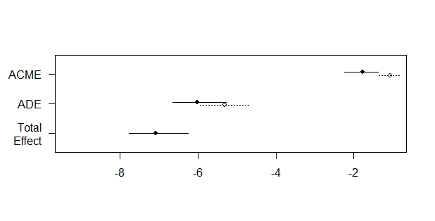
Figure 6.1: Plot of the 2-way decomposition (mediation package)
For the binary outcome:
mediation.res.death <- mediate(trad_m,                   # model of the mediator
                               trad_death_am,            # model of the outcome)
                               treat = "A0_PM2.5",       # exposure
                               mediator = "M_diabetes",  # mediator
                               robustSE = TRUE,          # estimate sandwich SEs
                               sims = 100)               # better to use >= 1000
summary(mediation.res.death)
#                          Estimate 95% CI Lower 95% CI Upper p-value
# ACME (control)            0.00860      0.00569         0.01  <2e-16 *** PNIE
# ACME (treated)            0.00979      0.00377         0.02  <2e-16 *** TNIE
# ADE (control)             0.06543      0.03658         0.09  <2e-16 *** PNDE
# ADE (treated)             0.06662      0.03946         0.09  <2e-16 *** TNDE
# Total Effect              0.07522      0.04800         0.10  <2e-16 ***
# Prop. Mediated (control)  0.11172      0.07323         0.18  <2e-16 ***
# Prop. Mediated (treated)  0.13066      0.05714         0.22  <2e-16 ***
# ACME (average)            0.00920      0.00567         0.01  <2e-16 ***
# ADE (average)             0.06603      0.03803         0.09  <2e-16 ***
# Prop. Mediated (average)  0.12119      0.07330         0.20  <2e-16 ***
Interestingly, the mediation package enable to carry-out a sensitivity analysis to test if unmeasured confounders of the mediator-outcome relationship could offset the estimated direct or indirect effects. This sensitivity analysis relies on assumptions on the mediator-outcome correlation coefficient. I.e., it can be used to test for unmeasured variables within the \(L(1)\) set in the causal structure of Figure 3.1.
If there exist unobserved (baseline) confounders of the M-Y relationship, we expect that \(\rho\) is no longer zero. The sensitivity analysis is conducted by varying the value of \(\rho\) and examining how the estimated ACME and ADE change.
Note 1: this sensitivity analysis cannot be used to test the assumption that no intermediate confounder \(L(1)\) of the mediator-outcome relationship is affected by the exposure (like in Figure 3.2).
Note 2: Sensitivity analysis from the mediation package cannot be applied when the mediator and the outcome are both binary. We will only use it for the “Quality of Life” outcome.
## Sensitivity analysis to test sequential ignorability (assess the possible
## existence of unobserved (baseline) confounders of the M-Y relationship)

## Estimate a probit model of the mediator
trad_m <- glm(M_diabetes ~ A0_PM2.5 + L0_male + L0_soc_env + L1,
              family = binomial("probit"), # sensitivity analysis works only for
                                           # probit models if M is binary
              data = df1_int)
mediation.res.qol <- mediate(trad_m,                   # model of the mediator
                             trad_qol_am,              # model of the outcome)
                             treat = "A0_PM2.5",       # exposure
                             mediator = "M_diabetes",  # mediator
                             robustSE = TRUE,          # estimate sandwich SEs
                             sims = 100)               # better to use >= 1000
summary(mediation.res.qol)
#                            Estimate 95% CI Lower 95% CI Upper p-value
#   ACME (control)             -1.071       -1.416        -0.79  <2e-16 ***
#   ACME (treated)             -1.784       -2.333        -1.31  <2e-16 ***
#   ADE (control)              -5.266       -5.809        -4.56  <2e-16 ***
#   ADE (treated)              -5.979       -6.515        -5.31  <2e-16 ***
#   Total Effect               -7.050       -7.754        -6.34  <2e-16 ***
#   Prop. Mediated (control)    0.151        0.119         0.19  <2e-16 ***
#   Prop. Mediated (treated)    0.254        0.194         0.32  <2e-16 ***
#   ACME (average)             -1.427       -1.889        -1.06  <2e-16 ***
#   ADE (average)              -5.623       -6.152        -4.97  <2e-16 ***
#   Prop. Mediated (average)    0.203        0.159         0.26  <2e-16 ***

sensisitivy <- medsens(mediation.res.qol,
                       rho.by = 0.1, # sensitivity parameter = correlation between
                       # the residuals of the mediator & outcome regressions
                       # here, rho varies from -0.9 to +0.9 by 0.1 increments
                       effect.type = "both", # "direct", "indirect" or "both"
                       sims = 100) # better to use >= 1000
summary(sensisitivy)
# Mediation Sensitivity Analysis: Average Mediation Effect
#   Sensitivity Region: ACME for Control Group
#         Rho ACME(control) 95% CI Lower 95% CI Upper R^2_M*R^2_Y* R^2_M~R^2_Y~
#   [1,] -0.6        0.0474      -0.0093       0.1229         0.36       0.2647
#
# Rho at which ACME for Control Group = 0: -0.6
# R^2_M*R^2_Y* at which ACME for Control Group = 0: 0.36
# R^2_M~R^2_Y~ at which ACME for Control Group = 0: 0.2647
#
# Rho at which ACME for Treatment Group = 0: -0.9
# R^2_M*R^2_Y* at which ACME for Treatment Group = 0: 0.81
# R^2_M~R^2_Y~ at which ACME for Treatment Group = 0: 0.5956
#
#   Mediation Sensitivity Analysis: Average Direct Effect
# Rho at which ADE for Control Group = 0: 0.8
# R^2_M*R^2_Y* at which ADE for Control Group = 0: 0.64
# R^2_M~R^2_Y~ at which ADE for Control Group = 0: 0.4706
#
# Rho at which ADE for Treatment Group = 0: 0.8
# R^2_M*R^2_Y* at which ADE for Treatment Group = 0: 0.64
# R^2_M~R^2_Y~ at which ADE for Treatment Group = 0: 0.4706

par(mfrow = c(2,2))
plot(sensisitivy)
par(mfrow = c(1,1))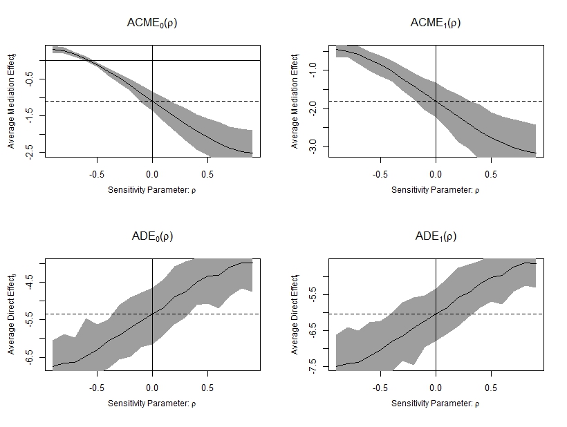
Figure 6.2: Sensitivity analysis testing unmeasured confounding of the M-Y relationship
Here, for the Pure Natural Indirect Effect:
- the confidence interval of the ACME (PNIE) contains zero when \(\rho=-0.6\);
- when the product of the residual variance explained by the omitted confounding is 0.36, the point estimate of PNIE = 0;
- when the product of the total variance explained by the omitted confounding is 0.27, the point estimate of PNIE = 0;
For the TNDE and PNDE,
- the confidence interval of the ADE (TNDE and PNDE) containt zero when \(\rho > +0.8\);
- when the product of the residual variance explained by the omitted confounding is 0.64, the point estimate of TNDE = 0;
- when the product of the total variance explained by the omitted confounding is 0.47, the point estimate of TNDE = 0;
We can conclude that the possibility of the PNIE and the TNIE cancelling out because of unmeasured M-Y confounding is unlikely in our example (it requires rather strong correlations).
6.4 Estimation of “Marginal” Randomized/Interventional Natural Direct (MRDE) and Indirect Effects (MRIE)
When we assume that the intermediate confounder \(L(1)\) of the \(M-Y\) relationship is affected by the exposure \(A\) (Causal model 2, Figure 3.2), an “interventional analogue” of the Average Total Effect decomposition into a Natural Direct and Indirect Effect has been suggested.(VanderWeele and Tchetgen Tchetgen 2017) (Lin et al. 2017) For these effects, counterfactual scenarios are defined by setting different values for the exposure (\(A = 0\) or \(A=1\)) and random draw in the distribution \(G_{A=a^\prime \mid L(0)}\) of the mediator (conditional on baseline counfounders \(L(0)\)) under the counterfactual scenario setting \(A=a^\prime\).
An Overall (Total) Effect can be defined by the contrast \(\text{OE} = \mathbb{E}\left[Y_{A=1,G_{A=1\mid L(0)}} \right] - \mathbb{E}\left[ Y_{A=0,G_{A=0\mid L(0)}} \right]\).
This Overall Effect can be decomposed into the sum of:
- a Marginal Randomised (or Interventional) Direct Effect: \(\text{MRDE}=\mathbb{E}\left[Y_{A=1,G_{A=0\mid L(0)}} \right] - \mathbb{E}\left[ Y_{A=0,G_{A=0\mid L(0)}} \right]\)
- a Marginal Randomised (or Interventional) Indirect Effect: \(\text{MRIE}=\mathbb{E}\left[Y_{A=1,G_{A=1\mid L(0)}} \right] - \mathbb{E}\left[ Y_{A=1,G_{A=0\mid L(0)}} \right]\)
For this 2-way decomposition, we have to estimate 3 causal quantities: \(\mathbb{E}\left[Y_{A=1,G_{A=1\mid L(0)}} \right]\), \(\mathbb{E}\left[ Y_{A=0,G_{A=0\mid L(0)}} \right]\) and \(\mathbb{E}\left[ Y_{A=1,G_{A=0\mid L(0)}} \right]\).
Under the identifiability conditions, in particular:
- no unmeasured exposure-outcome confounding
- no unmeasured mediator-outcome confounding
- and exposure-mediator confounding
the quantity of \(\mathbb{E}\left[Y_{a,G_{a^\prime\mid L(0)}} \right]\) can be estimated by the g-formula: \[\begin{multline*} \mathbb{E}\left[Y_{a,G_{a^\prime\mid L(0)}} \right]=\sum_{l(0),l(1),m} \mathbb{E}\left(Y \mid m,l(1),A=a,l(0),\right) \times P[L(1)=l(1) \mid a,l(0)] \\ \times P[M=m \mid a^\prime, l(0)] \times P(L(0)=l(0)) \end{multline*}\] These causal effects can be estimated by g-computation, IPTW, or TMLE. G-computation approaches are described below.
6.4.1 Parametric g-computation
The estimation using parametric g-computation is described in (Lin et al. 2017). The approach is described as an adaptation of the parametric g-computation presented for controlled direct effects, in order to estimate causal quantities \(\mathbb{E}(Y_{a,G_{a^\prime\mid L(0)}})\) corresponding to a counterfactual scenario where the exposures is set to \(A=a\) for all individuals and \(M\) is a random draw from the distribution \(G_{a^\prime \mid L(0)}\) of the mediator (conditional on \(L(0)\)) had the exposure been set to \(A=a^\prime\).
Estimation of \(\mathbb{E}(Y_{a,G_{a^\prime\mid L(0)}})\) relies on the following steps:
Fit parametric models for the time-varying confounders \(L(1)\), the mediator \(M\) and the outcome \(Y\) given the measured past;
Estimate the joint distribution of time-varying confounders (\(L(1)_{A=1}\) and \(L(1)_{A=0}\)) and of the mediator (\(M_{G_{A=0}}\) and \(M_{G_{A=1}}\)) under the counterfactual scenarios setting \(A = 1\) or \(A=0\);
Simulate the outcomes \(Y_{A=0,G_{A=0}}\), \(Y_{A=1,G_{A=1}}\) and \(Y_{A=1,G_{A=0}}\) in order to compute the randomized natural direct and indirect effects.
rm(list=ls())
df2_int <- read.csv(file = "data/df2_int.csv")

set.seed(54321)

# steps 1) to 3) will be repeated some fixed number k (for example k = 25)
# we will save the k results in a matrix of k rows and 4 columns for the randomized
# direct and indirect effects on death (binary) and QoL (continuous) outcomes
est <- matrix(NA, nrow = 25, ncol = 4)
colnames(est) <- c("rNDE.death", "rNIE.death", "rNDE.qol", "rNIE.qol")

# repeat k = 25 times the following steps 1) to 3)
for (k in 1:25) {
  ## 1) Fit parametric models for the time-varying confounders L(1), the mediator M
  ##    and the outcome Y
  ### 1a) fit parametric models of the confounders and mediators given the past
  L1.model <- glm(L1 ~ L0_male + L0_soc_env + A0_PM2.5,
                  family = "binomial", data = df2_int)
  M.model <- glm(M_diabetes ~ L0_male + L0_soc_env + A0_PM2.5 + L1,
                 family = "binomial", data = df2_int)
  ### 1b) fit parametric models of the outcomes given the past
  Y.death.model <- glm(Y_death ~ L0_male + L0_soc_env + A0_PM2.5 + L1 +
                         M_diabetes + A0_PM2.5:M_diabetes,
                       family = "binomial", data = df2_int)
  Y.qol.model <- glm(Y_qol ~ L0_male + L0_soc_env + A0_PM2.5 + L1 +
                       M_diabetes + A0_PM2.5:M_diabetes,
                     family = "gaussian", data = df2_int)

  ## 2) Estimate the joint distribution of time-varying confounders and of the
  ##    mediator under the counterfactual scenarios setting A0_PM2.5 = 1 or 0

  # set the exposure A0_PM2.5 to 0 or 1 in two new counterfactual data sets
  data.A0  <- data.A1 <- df2_int
  data.A0$A0_PM2.5 <- 0
  data.A1$A0_PM2.5 <- 1
  # simulate L1 values under the counterfactual exposures A0_PM2.5=0 or A0_PM2.5=1
  p.L1.A0 <- predict(L1.model, newdata = data.A0, type="response")
  p.L1.A1 <- predict(L1.model, newdata = data.A1, type="response")
  sim.L1.A0 <- rbinom(n = nrow(df2_int), size = 1, prob = p.L1.A0)
  sim.L1.A1 <- rbinom(n = nrow(df2_int), size = 1, prob = p.L1.A1)

  # replace L(1) by their counterfactual values in the data under A=0 or A=1
  data.A0.L <- data.A0
  data.A1.L <- data.A1
  data.A0.L$L1 <- sim.L1.A0
  data.A1.L$L1 <- sim.L1.A1

  # simulate M values under the counterfactual exposures A0_PM2.5=0 or A0_PM2.5=1
  p.M.A0 <- predict(M.model, newdata = data.A0.L, type="response")
  p.M.A1 <- predict(M.model, newdata = data.A1.L, type="response")
  sim.M.A0 <- rbinom(n = nrow(df2_int), size = 1, prob = p.M.A0)
  sim.M.A1 <- rbinom(n = nrow(df2_int), size = 1, prob = p.M.A1)
  # permute the n values of the joint mediator to obtain the random distributions
  # of the mediator: G_{A=0} and G_{A=1}
  marg.M.A0 <- sample(sim.M.A0, replace = FALSE)
  marg.M.A1 <- sample(sim.M.A1, replace = FALSE)

  ## 3) Simulate the outcomes Y_{A=0,G_{A=0}}
  ### 3a) use the previous permutation to replace the mediator
  ### in the counterfactual data sets for Y_{A=0,G_{A=0}}, Y_{A=1,G_{A=1}} and
  ### Y_{A=1,G_{A=0}}
  data.A0.G0 <- data.A0.G1 <- data.A0.L
  data.A1.G0 <- data.A1.G1 <- data.A1.L

  data.A0.G0$M_diabetes <- marg.M.A0
  # data.A0.G1$M_diabetes <- marg.M.A1 # note: this data set will not be useful

  data.A1.G0$M_diabetes <- marg.M.A0
  data.A1.G1$M_diabetes <- marg.M.A1

  # simulate the average outcome using the models fitted at step 1)
  p.death.A1.G1 <- predict(Y.death.model, newdata = data.A1.G1, type="response")
  p.death.A1.G0 <- predict(Y.death.model, newdata = data.A1.G0, type="response")
  p.death.A0.G0 <- predict(Y.death.model, newdata = data.A0.G0, type="response")

  m.qol.A1.G1 <- predict(Y.qol.model, newdata = data.A1.G1, type="response")
  m.qol.A1.G0 <- predict(Y.qol.model, newdata = data.A1.G0, type="response")
  m.qol.A0.G0 <- predict(Y.qol.model, newdata = data.A0.G0, type="response")

  ## save the results in row k
  # rNDE = E(Y_{A=1,G_{A=0}}) - E(Y_{A=0,G_{A=0}})
  # rNIE = E(Y_{A=1,G_{A=1}}) - E(Y_{A=1,G_{A=0}})
  est[k,"rNDE.death"]<- mean(p.death.A1.G0) - mean(p.death.A0.G0)
  est[k,"rNIE.death"] <- mean(p.death.A1.G1) - mean(p.death.A1.G0)

  est[k,"rNDE.qol"] <- mean(m.qol.A1.G0) - mean(m.qol.A0.G0)
  est[k,"rNIE.qol"] <- mean(m.qol.A1.G1) - mean(m.qol.A1.G0)
}

# take empirical mean of final predicted outcomes
rNDE.death <- mean(est[,"rNDE.death"])
rNDE.death
# [1] 0.07118987
rNIE.death <- mean(est[,"rNIE.death"])
rNIE.death
# [1] 0.0110088

rNDE.qol <- mean(est[,"rNDE.qol"])
rNDE.qol
# [1] -6.649923
rNIE.qol <-  mean(est[,"rNIE.qol"])
rNIE.qol
# [1] -1.585373
In this example,
- the marginal “randomized” Natural Direct and Indirect effect on death are a \(MRDE \approx +7.1\%\) and \(MRIE \approx +1.1\%\);
- the marginal “randomized” Natural Direct and Indirect effect on quality of life are a \(MRDE \approx -6.6\) and \(MRIE \approx -1.6\);
95% confidence intervals can be calculated by repeating the algorithm in >500 bootstrap samples of the original data set.
6.4.2 G-computation by iterative conditional expectation
We describe below the g-computation algorithm which is used in the stremr package (“Streamlined Causal Inference for Static, Dynamic and Stochastic Regimes in Longitudinal Data”).
Note that G-computation by iterative expectation is preferable if the set of intermediate confounders \(L(1)\) is high-dimensional as we only need to fit 1 model by counterfactual scenario in the procedure described below (whatever the dimensionaly of the set \(L(1)\)), whereas at least 1 model by \(L(1)\) variable and by counterfactual scenario are needed with parametric g-computation.
The following 4 steps are applied:
Fit a parametric model for the mediator conditional on \(A\) and \(L(0)\). This model will be used to predict the probabilities \(G_{A=0|L(0)}=P(M=1|A=0,L(0))\) and \(G_{A=1|L(0)}=P(M=1|A=1,L(0))\) under the counterfactual scenarios setting \(A=0\) and \(A=1\).
Fit parametric models for the outcome \(Y\) given the past and generate predicted values \(\bar{Q}_{L(2)}(M=0)\) and \(\bar{Q}_{L(2)}(M=1)\) by evaluating the regression setting the mediator value to \(M=0\) or to \(M=1\).
Then calculate a weighted sum of the predicted \(\bar{Q}_{L(2)}(M)\), with weights given by \(G_{A=1|L(0)}\) or \(G_{A=0|L(0)}\): \[\begin{align*} \bar{Q}_{L(2),G_{A=0 \mid L(0)}} &= \bar{Q}_{L(2)}(M=1) \times G_{A=0|L(0)} + \bar{Q}_{L(2)}(M=0) \times \left[1 - G_{A=0 \mid L(0)} \right] \\ \bar{Q}_{L(2),G_{A=1 \mid L(0)}} &= \bar{Q}_{L(2)}(M=1) \times G_{A=1|L(0)} + \bar{Q}_{L(2)}(M=0) \times \left[1 - G_{A=1 \mid L(0)} \right] \end{align*}\]
Fit parametric models for the predicted values \(\bar{Q}_{L(2),G_{A=a \mid L(0)}}\) conditional on the exposure \(A\) and baseline confounders \(L(0)\), and generate predicted values \(\bar{Q}_{L(1),G_{A=0 \mid L(0)}}(A=0)\), \(\bar{Q}_{L(1),G_{A=0 \mid L(0)}}(A=1)\) and \(\bar{Q}_{L(1),G_{A=1 \mid L(0)}}(A=1)\).
Estimate the marginal randomized natural direct and indirect effects, using the means of the \(\bar{Q}_{L(1),G_{A=a^\prime \mid L(0)}}(A=a)\) calculated at the previous step
\[\begin{align*} \text{MRDE}_\text{ICE.gcomp} &= \frac{1}{n} \sum_{i=1}^n \left[ \bar{Q}_{L(1),G_{A=0 \mid L(0)}}(A=1) \right] - \frac{1}{n} \sum_{i=1}^n \left[ \bar{Q}_{L(1),G_{A=0 \mid L(0)}}(A=0) \right] \\ \text{MRIE}_\text{ICE.gcomp} &= \frac{1}{n} \sum_{i=1}^n \left[ \bar{Q}_{L(1),G_{A=1 \mid L(0)}}(A=1) \right] - \frac{1}{n} \sum_{i=1}^n \left[ \bar{Q}_{L(1),G_{A=0 \mid L(0)}}(A=1) \right] \\ \end{align*}\]
rm(list=ls())
df2_int <- read.csv(file = "data/df2_int.csv")

## 1) Fit a parametric model for the mediator conditional on A and L(0)
##    and generate predicted values by evaluating the regression setting the exposure
##    value to A=0 or A=1
### 1a) Fit parametric models for the mediator M, conditional on the exposure A and
###    baseline confounder Pr(M=1|A,L(0)) (but not conditional on L(1))
G.model <- glm(M_diabetes ~ L0_male + L0_soc_env + A0_PM2.5,
               family = "binomial", data = df2_int)

### 1b) generate predicted probabilites by evaluating the regression setting the
###     exposure value to A=0 or to A=1
# create datasets corresponding to the counterfactual scenarios setting A=0 and A=1
data.Ais0  <- data.Ais1 <- df2_int
data.Ais0$A0_PM2.5 <- 0
data.Ais1$A0_PM2.5 <- 1

# estimate G_{A=0|L(0)} = Pr(M=1|A=0,L(0)) and G_{A=1|L(0)} = Pr(M=1|A=1,L(0))
G.Ais0.L0 <-predict(G.model, newdata = data.Ais0, type="response")
G.Ais1.L0 <-predict(G.model, newdata = data.Ais1, type="response")

## 2) Fit parametric models for the observed data for the outcome Y given the past
##    and generate predicted values by evaluating the regression setting the mediator
##    value to M=0 or to M=1
##    then calculate a weighted sum of the predicted Q.L2, with weights given by G
### 2a) fit parametric models of the outcomes given the past
Y.death.model <- glm(Y_death ~ L0_male + L0_soc_env + A0_PM2.5 + L1 +
                       M_diabetes + A0_PM2.5:M_diabetes,
                     family = "binomial", data = df2_int)
Y.qol.model <- glm(Y_qol ~ L0_male + L0_soc_env + A0_PM2.5 + L1 +
                     M_diabetes + A0_PM2.5:M_diabetes,
                   family = "gaussian", data = df2_int)

### 2b) generate predicted values by evaluating the regression setting the mediator
###     value to M=0 or to M=1
data.Mis0  <- data.Mis1 <- df2_int
data.Mis0$M_diabetes <- 0
data.Mis1$M_diabetes <- 1

Q.L2.death.Mis0 <- predict(Y.death.model, newdata = data.Mis0, type="response")
Q.L2.death.Mis1 <- predict(Y.death.model, newdata = data.Mis1, type="response")

Q.L2.qol.Mis0 <- predict(Y.qol.model, newdata = data.Mis0, type="response")
Q.L2.qol.Mis1 <- predict(Y.qol.model, newdata = data.Mis1, type="response")

### 2c) calculate a weighted sum of the predicted Q.L2, with weights given by the
###     predicted probabilities of the mediator G_{A=0|L(0)} or G_{A=1|L(0)}
# calculate barQ.L2_{A=0,G_{A=0|L(0)}}
Q.L2.death.A0.G0 <- Q.L2.death.Mis1 * G.Ais0.L0 + Q.L2.death.Mis0 * (1 - G.Ais0.L0)
Q.L2.qol.A0.G0 <- Q.L2.qol.Mis1 * G.Ais0.L0 + Q.L2.qol.Mis0 * (1 - G.Ais0.L0)

# calculate barQ.L2_{A=1,G_{A=0|L(0)}}
# note at this step, quantities are similar to barQ.L2_{A=0,G_{A=0|L(0)}}
Q.L2.death.A1.G0 <- Q.L2.death.Mis1 * G.Ais0.L0 + Q.L2.death.Mis0 * (1 - G.Ais0.L0)
Q.L2.qol.A1.G0 <- Q.L2.qol.Mis1 * G.Ais0.L0 + Q.L2.qol.Mis0 * (1 - G.Ais0.L0)

# calculate barQ.L2_{A=1,G_{A=1|L(0)}}
Q.L2.death.A1.G1 <- Q.L2.death.Mis1 * G.Ais1.L0 + Q.L2.death.Mis0 * (1 - G.Ais1.L0)
Q.L2.qol.A1.G1 <- Q.L2.qol.Mis1 * G.Ais1.L0 + Q.L2.qol.Mis0 * (1 - G.Ais1.L0)

## 3) Fit parametric models for the predicted values barQ.L2 conditional on the
##    exposure A and baseline confounders L(0)
##    and generate predicted values by evaluating the regression setting the exposure
##    value to A=0 or to A=1
### 3a) Fit parametric models for the predicted values barQ.L2 conditional on the
###    exposure A and baseline confounders L(0)
L1.death.A0.G0.model <- glm(Q.L2.death.A0.G0 ~ L0_male + L0_soc_env + A0_PM2.5,
                            family = "quasibinomial", data = df2_int)
L1.death.A1.G0.model <- glm(Q.L2.death.A1.G0 ~ L0_male + L0_soc_env + A0_PM2.5,
                            family = "quasibinomial", data = df2_int)
L1.death.A1.G1.model <- glm(Q.L2.death.A1.G1 ~ L0_male + L0_soc_env + A0_PM2.5,
                            family = "quasibinomial", data = df2_int)

L1.qol.A0.G0.model <- glm(Q.L2.qol.A0.G0 ~ L0_male + L0_soc_env + A0_PM2.5,
                          family = "gaussian", data = df2_int)
L1.qol.A1.G0.model <- glm(Q.L2.qol.A1.G0 ~ L0_male + L0_soc_env + A0_PM2.5,
                          family = "gaussian", data = df2_int)
L1.qol.A1.G1.model <- glm(Q.L2.qol.A1.G1 ~ L0_male + L0_soc_env + A0_PM2.5,
                          family = "gaussian", data = df2_int)

### 3b) generate predicted values by evaluating the regression setting the exposure
###     value to A=0 or to A=1
Q.L1.death.A0.G0 <- predict(L1.death.A0.G0.model, newdata = data.Ais0, type="response")
Q.L1.death.A1.G0 <- predict(L1.death.A1.G0.model, newdata = data.Ais1, type="response")
Q.L1.death.A1.G1 <- predict(L1.death.A1.G1.model, newdata = data.Ais1, type="response")

Q.L1.qol.A0.G0 <- predict(L1.qol.A0.G0.model, newdata = data.Ais0, type="response")
Q.L1.qol.A1.G0 <- predict(L1.qol.A1.G0.model, newdata = data.Ais1, type="response")
Q.L1.qol.A1.G1 <- predict(L1.qol.A1.G1.model, newdata = data.Ais1, type="response")

## 4) Estimate the marginal randomized natural direct and indirect effects
### MRDE = E(Y_{A=1,G_{A=0|L(0)}}) - E(Y_{A=0,G_{A=0|L(0)}})
### MRIE = E(Y_{A=1,G_{A=1|L(0)}}) - E(Y_{A=1,G_{A=0|L(0)}})

### for deaths:
MRDE.death <- mean(Q.L1.death.A1.G0) - mean(Q.L1.death.A0.G0)
MRDE.death
# [1] 0.0714693
MRIE.death <- mean(Q.L1.death.A1.G1) - mean(Q.L1.death.A1.G0)
MRIE.death
# [1] 0.01130057

### for quality of life
MRDE.qol <- mean(Q.L1.qol.A1.G0) - mean(Q.L1.qol.A0.G0)
MRDE.qol
# [1] -6.719193
MRIE.qol <-  mean(Q.L1.qol.A1.G1) - mean(Q.L1.qol.A1.G0)
MRIE.qol
# [1] -1.624645
Results are close to the estimations obtained previously with parametric g-computation.
- the marginal “randomized” Natural Direct and Indirect effect on death are a \(MRDE \approx +7.1\%\) and \(MRIE \approx +1.1\%\);
- the marginal “randomized” Natural Direct and Indirect effect on quality of life are a \(MRDE \approx -6.6\) and \(MRIE \approx -1.6\);
95% confidence intervals can be calculated by bootstrap.
6.5 Using the CMAverse package for 2-way, 3-way and 4-way decomposition
The CMAverse package can be used to estimate the 2-way, 3-way and 4-way decompositions of a total effect by parametric g-computation, whether the intermediate confounder \(L(1)\) of the \(M-Y\) relationship is affected by the exposure \(A\) or not.
Here is an example with a continuous outcome using the cmest function. Note that :
- parametric g-computation is applied by specifying
model = "gformula". Theestimationargument should be set toimputation(as the counterfactual values will be imputed). - the presence of intermediate confounder \(L(1)\) of the \(M-Y\) relationship affected by the exposure \(A\) can be specified using the
postcregargument, - the presence of an \(A \ast M\) interaction effect on the outcome is indicated using the
EMintargument, - for the estimation of the Controlled direct effect, the fixed value set for the mediator is indicated using the
mvalargument.
The function returns the following results:
- fit of the Outcome regression \(\overline{Q}_Y = \mathbb{E}(Y \mid L(0),A,L(1),M)\),
- fit of the Mediator regression \(g_A = P(M=1 \mid L(0),A,L(1))\),
- fit of the intermediate confounder regression \(\overline{Q}_{L(1)} = P(L(1)=1\mid L(0),A)\),
- the 2-way, 3-way and 4-way decompositions.
library(CMAverse)
rm(list=ls())
df2_int <- read.csv(file = "data/df2_int.csv")

set.seed(1234)
res_gformula_Qol_M0 <- cmest(data = df2_int,
                         model = "gformula", # for parametric g-computation
                         outcome = "Y_qol", # outcome variable
                         exposure = "A0_PM2.5", # exposure variable
                         mediator = "M_diabetes", # mediator
                         basec = c("L0_male",     # confounders
                                   "L0_soc_env"),
                         postc = "L1", # intermediate confounder (post-exposure)
                         EMint = TRUE, # exposures*mediator interaction
                         mreg = list("logistic"), # g(M=1|L1,A,L0)
                         yreg = "linear",# Qbar.L2 = P(Y=1|M,L1,A,L0)
                         postcreg = list("logistic"), # Qbar.L1 = P(L1=1|A,L0)
                         astar = 0,
                         a = 1,
                         mval = list(0), # do(M=0) to estimate CDE_m
                         estimation = "imputation", # if model= gformula
                         inference = "bootstrap",
                         boot.ci.type = "per", # for percentile, other option: "bca"
                         nboot = 2) # we should use a large number of bootstrap samples
summary(res_gformula_Qol_M0)

### 1) Estimation of Qbar.Y = P(Y=1|M,L1,A,L0) with A*M interaction,
### Outcome regression:
# Call:
#   glm(formula = Y_qol ~ A0_PM2.5 + M_diabetes + A0_PM2.5 * M_diabetes +
#         L0_male + L0_soc_env + L1, family = gaussian(),
#       data = getCall(x$reg.output$yreg)$data, weights = getCall(x$reg.output$yreg)$weights)
# Coefficients:
#                         Estimate Std. Error t value Pr(>|t|)
#   (Intercept)            74.8247     0.2133 350.823  < 2e-16 ***
#   A0_PM2.5               -3.7014     0.4295  -8.617  < 2e-16 ***
#   M_diabetes             -8.6336     0.2331 -37.042  < 2e-16 ***
#   L0_male                -0.7280     0.2019  -3.605 0.000313 ***
#   L0_soc_env             -2.8828     0.2116 -13.621  < 2e-16 ***
#   L1                     -5.1668     0.2189 -23.608  < 2e-16 ***
#   A0_PM2.5:M_diabetes    -5.5119     0.6440  -8.559  < 2e-16 ***

### 2) Estimation of g(M=1|L1,A,L0), model of the mediator
### Mediator regressions:
# Call:
#   glm(formula = M_diabetes ~ A0_PM2.5 + L0_male + L0_soc_env +
#         L1, family = binomial(), data = getCall(x$reg.output$mreg[[1L]])$data,
#       weights = getCall(x$reg.output$mreg[[1L]])$weights)
# Coefficients:
#                         Estimate Std. Error z value Pr(>|z|)
#   (Intercept)           -1.36249    0.04783 -28.488  < 2e-16 ***
#   A0_PM2.5               0.30994    0.06668   4.648 3.35e-06 ***
#   L0_male                0.24661    0.04369   5.644 1.66e-08 ***
#   L0_soc_env             0.30628    0.04650   6.587 4.50e-11 ***
#   L1                     0.86045    0.04493  19.152  < 2e-16 ***

### 3) Estimation of Qbar.L1 = P(L1=1|A,L0), model of intermediate confounder
### Regressions for mediator-outcome confounders affected by the exposure:
# Call:
#   glm(formula = L1 ~ A0_PM2.5 + L0_male + L0_soc_env,
#       family = binomial(), data = getCall(x$reg.output$postcreg[[1L]])$data,
#       weights = getCall(x$reg.output$postcreg[[1L]])$weights)
#
# Coefficients:
#                         Estimate Std. Error z value Pr(>|z|)
#   (Intercept)           -0.86983    0.04292 -20.267  < 2e-16 ***
#   A0_PM2.5               0.94354    0.06475  14.572  < 2e-16 ***
#   L0_male               -0.19827    0.04289  -4.622 3.80e-06 ***
#   L0_soc_env             0.32047    0.04556   7.034 2.01e-12 ***

### 4) Effect decomposition on the mean difference scale via the g-formula approach
#
# Direct counterfactual imputation estimation with
# bootstrap standard errors, percentile confidence intervals and p-values
#
#                  Estimate Std.error   95% CIL 95% CIU  P.val
#   cde           -5.863750  0.233488 -4.933234  -4.620 <2e-16 ***
#   rpnde         -7.565835  0.199867 -6.689581  -6.421 <2e-16 ***
#   rtnde         -8.463729  0.157383 -7.266085  -7.055 <2e-16 ***
#   rpnie         -1.406410  0.021876 -0.971101  -0.942 <2e-16 ***
#   rtnie         -2.304304  0.064359 -1.604682  -1.518 <2e-16 ***
#   te            -9.870139  0.135507 -8.207796  -8.026 <2e-16 ***
#   rintref       -1.702085  0.033622 -1.801518  -1.756 <2e-16 ***
#   rintmed       -0.897894  0.042484 -0.633581  -0.577 <2e-16 ***
#   cde(prop)      0.594090  0.018945  0.575575   0.601 <2e-16 ***
#   rintref(prop)  0.172448  0.007802  0.213991   0.224 <2e-16 ***
#   rintmed(prop)  0.090971  0.006479  0.070244   0.079 <2e-16 ***
#   rpnie(prop)    0.142491  0.004663  0.114737   0.121 <2e-16 ***
#   rpm            0.233462  0.011142  0.184981   0.200 <2e-16 ***
#   rint           0.263419  0.014282  0.284235   0.303 <2e-16 ***
#   rpe            0.405910  0.018945  0.398973   0.424 <2e-16 ***
#   ---
#   Signif. codes:  0 ‘***’ 0.001 ‘**’ 0.01 ‘*’ 0.05 ‘.’ 0.1 ‘ ’ 1
#
# cde: controlled direct effect;
# rpnde: randomized analogue of pure natural direct effect;
# rtnde: randomized analogue of total natural direct effect;
# rpnie: randomized analogue of pure natural indirect effect;
# rtnie: randomized analogue of total natural indirect effect;
# te: total effect; rintref: randomized analogue of reference interaction;
# rintmed: randomized analogue of mediated interaction;
# cde(prop): proportion cde;
# rintref(prop): proportion rintref;
# rintmed(prop): proportion rintmed;
# rpnie(prop): proportion rpnie;
# rpm: randomized analogue of overall proportion mediated;
# rint: randomized analogue of overall proportion attributable to interaction;
# rpe: randomized analogue of overall proportion eliminated
Using the CMAverse package,
- the total effect (overall effect) on the QoL quantitative outcome is estimated to be \(TE = \mathbb{E}\left(Y_{A=1,G_{A=1\mid L(0)}} \right) - \mathbb{E}\left(Y_{A=0,G_{A=0\mid L(0)}} \right) \approx -9.87\),
- the controlled direct effect (\(CDE_{M=0}\)), setting \(M=0\) is \(CDE_{M=0}=\mathbb{E}\left(Y_{A=1,M=0} \right) - \mathbb{E}\left(Y_{A=0,M=0} \right)\approx -5.86\),
- the randomized pure natural direct effect is \(rPNDE = \mathbb{E}\left(Y_{A=1,G_{A=0\mid L(0)}} \right) - \mathbb{E}\left(Y_{A=0,G_{A=0\mid L(0)}} \right)\approx -7.57\)
- the randomized total natural indirect effect is \(rTNIE = \mathbb{E}\left(Y_{A=1,G_{A=1\mid L(0)}} \right) - \mathbb{E}\left(Y_{A=1,G_{A=0\mid L(0)}} \right)\approx -2.30\)
(VanderWeele 2014) defined the 3-way or 4-way decomposition in causal structures with no intermediate confounder \(L(1)\) of the \(M-Y\) relationship affected by the exposure \(A\). In causal structures with such intermediate confounders (Causal model 2, Figure 3.2), analogues of the 3-way and 4-way decomposition can still be defined. Those analogues are estimated by the CMAverse package. They can be calculated from the controlled direct effect (setting \(M=0\)) and the pure Natural Direct and Indirect Effects, using the following relationships:
- We can start by estimating the Total Effect (Overall effect), the CDE (setting \(M=0\)), the randomized Pure Natural Direct effect and the randomized Pure Natural Indirect Effect: \[\begin{align*} TE &= \mathbb{E}\left(Y_{A=1,G_{A=1\mid L(0)}} \right) - \mathbb{E}\left(Y_{A=0,G_{A=0\mid L(0)}} \right) \\ CDE_{M=0} &=\mathbb{E}\left(Y_{A=1,M=0} \right) - \mathbb{E}\left(Y_{A=0,M=0} \right) \\ rPNDE &= \mathbb{E}\left(Y_{A=1,G_{A=0\mid L(0)}} \right) - \mathbb{E}\left(Y_{A=0,G_{A=0\mid L(0)}} \right) \\ rPNIE &= \mathbb{E}\left(Y_{A=0,G_{A=1\mid L(0)}} \right) - \mathbb{E}\left(Y_{A=0,G_{A=0\mid L(0)}} \right) \end{align*}\]
- the Mediated Interaction can then be obtained by : \[\begin{align*} MIE &= rTNDE - rPNDE = rTNIE - rPNIE \\ MIE &= \left[\mathbb{E}\left(Y_{A=1,G_{A=1\mid L(0)}} \right) - \mathbb{E}\left(Y_{A=0,G_{A=1\mid L(0)}} \right)\right] \\ & \quad \quad - \left[\mathbb{E}\left(Y_{A=1,G_{A=0\mid L(0)}} \right) - \mathbb{E}\left(Y_{A=1,G_{A=0\mid L(0)}} \right)\right] \\ &= \left[\mathbb{E}\left(Y_{A=1,G_{A=1\mid L(0)}} \right) - \mathbb{E}\left(Y_{A=1,G_{A=0\mid L(0)}} \right)\right] \\ & \quad \quad - \left[\mathbb{E}\left(Y_{A=0,G_{A=1\mid L(0)}} \right) - \mathbb{E}\left(Y_{A=0,G_{A=0\mid L(0)}} \right)\right] \end{align*}\]
- and the Reference Interaction can be obtained by : \[\begin{align*} RIE &= rPNDE - CDE_{M=0} \\ RIE &= \left[\mathbb{E}\left(Y_{A=1,G_{A=0\mid L(0)}} \right) - \mathbb{E}\left(Y_{A=0,G_{A=0\mid L(0)}} \right) \right] - \left[ \mathbb{E}\left(Y_{A=1,M=0} \right) - \mathbb{E}\left(Y_{A=0,M=0} \right) \right] \end{align*}\]
## Using the previous results, we can check those equalities for the analogues
## of the 3-way and 4-way decomposition
res_gformula_Qol_M0$effect.pe["te"]
# TE = -9.870139
res_gformula_Qol_M0$effect.pe["cde"]
# CDE(M=0) = -5.86375
res_gformula_Qol_M0$effect.pe["rpnde"]
# rPNDE = -7.565835
res_gformula_Qol_M0$effect.pe["rpnie"]
# rPNIE = -1.40641

## Check that MI = rTNIE - rPNIE = rTNDE - rPNDE
(res_gformula_Qol_M0$effect.pe["rtnie"] - res_gformula_Qol_M0$effect.pe["rpnie"])
# -0.897894
(res_gformula_Qol_M0$effect.pe["rtnde"] - res_gformula_Qol_M0$effect.pe["rpnde"])
# -0.897894
res_gformula_Qol_M0$effect.pe["rintmed"]
# -0.897894 # we have MI = rTNIE - rPNIE = rTNDE - rPNDE

## Check that RE = PNDE - CDE_{M=0}
res_gformula_Qol_M0$effect.pe["rpnde"] - res_gformula_Qol_M0$effect.pe["cde"]
# -1.702085
res_gformula_Qol_M0$effect.pe["rintref"]
# -1.702085 # we have RE = PNDE - CDE_{M=0}
With a binary outcome, we can use the same cmest function as previously, replacing the yreg = "linear" argument by yreg = "logistic". The results will be given on the Odds Ratio scale:
set.seed(1234)
res_gformula_OR_M0 <- cmest(data = df2_int,
                      model = "gformula",
                      outcome = "Y_death",
                      exposure = "A0_PM2.5",
                      mediator = "M_diabetes",
                      basec = c("L0_male", "L0_soc_env"),
                      postc = "L1",
                      EMint = TRUE,
                      mreg = list("logistic"), # g(M=1|L1,A,L0)
                      yreg = "logistic",# Qbar.L2 = P(Y=1|M,L1,A,L0)
                      postcreg = list("logistic"), # Qbar.L1 = P(L1=1|A,L0)
                      astar = 0,
                      a = 1,
                      mval = list(0), # do(M=0) to estimate CDE_m
                      estimation = "imputation", # parametric g-comp if model= gformula
                      inference = "bootstrap",
                      boot.ci.type = "per", # forpercentile, other option: "bca"
                      nboot = 2) # we should use a large number of bootstrap samples
summary(res_gformula_OR_M0)
### 1) Estimation of Qbar.Y = P(Y=1|M,L1,A,L0) with A*M interaction,
###    by logistic regression
# Outcome regression:
# Call:
# glm(formula = Y_death ~ A0_PM2.5 + M_diabetes + A0_PM2.5 * M_diabetes +
#     L0_male + L0_soc_env + L1, family = binomial(),
#     data = getCall(x$reg.output$yreg)$data, weights = getCall(x$reg.output$yreg)$weights)
#
# Coefficients:
#                       Estimate Std. Error z value Pr(>|z|)
# (Intercept)           -2.04033    0.05855 -34.849  < 2e-16 ***
# A0_PM2.5               0.28922    0.10123   2.857  0.00428 **
# M_diabetes             0.44406    0.05569   7.974 1.53e-15 ***
# L0_male                0.26913    0.04996   5.387 7.15e-08 ***
# L0_soc_env             0.34603    0.05432   6.370 1.89e-10 ***
# L11                    0.42894    0.05195   8.257  < 2e-16 ***
# A0_PM2.5:M_diabetes    0.04387    0.14311   0.307  0.75919

# etc

### 4) Effect decomposition on the odds ratio scale via the g-formula approach
#                 Estimate Std.error  95% CIL 95% CIU  P.val
# Rcde            1.592115  0.121242 1.401748   1.565 <2e-16 ***
# rRpnde          1.610141  0.064880 1.458433   1.546 <2e-16 ***
# rRtnde          1.621371  0.046720 1.479227   1.542 <2e-16 ***
# rRpnie          1.076471  0.001714 1.036683   1.039 <2e-16 ***
# rRtnie          1.083979  0.014539 1.034267   1.054 <2e-16 ***
# Rte             1.745359  0.045898 1.536897   1.599 <2e-16 ***
# ERcde           0.392219  0.073776 0.277167   0.376 <2e-16 ***
# rERintref       0.217921  0.008895 0.169383   0.181 <2e-16 ***
# rERintmed       0.058747  0.017268 0.016243   0.039 <2e-16 ***
# rERpnie         0.076471  0.001714 0.036684   0.039 <2e-16 ***
# ERcde(prop)     0.526216  0.083694 0.515858   0.628 <2e-16 ***
# rERintref(prop) 0.292371  0.040769 0.283120   0.338 <2e-16 ***
# rERintmed(prop) 0.078817  0.034491 0.027264   0.074 <2e-16 ***
# rERpnie(prop)   0.102596  0.008434 0.061314   0.073 <2e-16 ***
# rpm             0.181413  0.042925 0.088578   0.146 <2e-16 ***
# rint            0.371188  0.075260 0.310384   0.411 <2e-16 ***
# rpe             0.473784  0.083694 0.371698   0.484 <2e-16 ***
# ---
# Signif. codes:  0 ‘***’ 0.001 ‘**’ 0.01 ‘*’ 0.05 ‘.’ 0.1 ‘ ’ 1
#
# Rcde: controlled direct effect odds ratio;
# rRpnde: randomized analogue of pure natural direct effect odds ratio;
# rRtnde: randomized analogue of total natural direct effect odds ratio;
# rRpnie: randomized analogue of pure natural indirect effect odds ratio;
# rRtnie: randomized analogue of total natural indirect effect odds ratio;
# Rte: total effect odds ratio;
# ERcde: excess relative risk due to controlled direct effect;
# rERintref: randomized analogue of excess relative risk due to reference interaction;
# rERintmed: randomized analogue of excess relative risk due to mediated interaction;
# rERpnie: randomized analogue of excess relative risk due to pure natural indirect effect;
# ERcde(prop): proportion ERcde;
# rERintref(prop): proportion rERintref;
# rERintmed(prop): proportion rERintmed;
# rERpnie(prop): proportion rERpnie;
# rpm: randomized analogue of overall proportion mediated;
# rint: randomized analogue of overall proportion attributable to interaction;
# rpe: randomized analogue of overall proportion eliminated)
If we prefer to estimate results for the binary outcome on a risk difference scale, it is still possible, by appyling a linear regression for the outcome model, using the argument yreg = "linear".
set.seed(1234)
res_gformula_RD_M0 <- cmest(data = df2_int,
                      model = "gformula",
                      outcome = "Y_death",
                      exposure = "A0_PM2.5",
                      mediator = "M_diabetes",
                      basec = c("L0_male", "L0_soc_env"),
                      postc = "L1",
                      EMint = TRUE,
                      mreg = list("logistic"), # g(M=1|L1,A,L0)
                      yreg = "linear",# Qbar.L2 = P(Y=1|M,L1,A,L0)
                      postcreg = list("logistic"), # Qbar.L1 = P(L1=1|A,L0)
                      astar = 0,
                      a = 1,
                      mval = list(0), # do(M=0) to estimate CDE_m
                      estimation = "imputation", # parametric g-comp if model= gformula
                      inference = "bootstrap",
                      boot.ci.type = "per", # forpercentile, other option: "bca"
                      nboot = 2) # we should use a large number of bootstrap samples
summary(res_gformula_RD_M0)
## 4) Effect decomposition on the mean difference scale via the g-formula approach
# Direct counterfactual imputation estimation with
# bootstrap standard errors, percentile confidence intervals and p-values
#
# Direct counterfactual imputation estimation with
# bootstrap standard errors, percentile confidence intervals and p-values
#
#                  Estimate Std.error   95% CIL 95% CIU  P.val
#   cde           0.0638914 0.0158641 0.0467659   0.068 <2e-16 ***
#   rpnde         0.0734700 0.0307357 0.0598528   0.101 <2e-16 ***
#   rtnde         0.0771555 0.0333264 0.0647151   0.109 <2e-16 ***
#   rpnie         0.0090890 0.0033498 0.0050769   0.010 <2e-16 ***
#   rtnie         0.0127744 0.0007591 0.0134198   0.014 <2e-16 ***
#   te            0.0862445 0.0299766 0.0742924   0.115 <2e-16 ***
#   rintref       0.0095786 0.0148716 0.0130869   0.033 <2e-16 ***
#   rintmed       0.0036855 0.0025907 0.0048623   0.008 <2e-16 ***
#   cde(prop)     0.7408176 0.0263715 0.5945733   0.630 <2e-16 ***
#   rintref(prop) 0.1110634 0.0841501 0.1744983   0.288 <2e-16 ***
#   rintmed(prop) 0.0427328 0.0055167 0.0653396   0.073 <2e-16 ***
#   rpnie(prop)   0.1053862 0.0632953 0.0451212   0.130 <2e-16 ***
#   rpm           0.1481190 0.0577786 0.1178726   0.195 <2e-16 ***
#   rint          0.1537963 0.0896668 0.2398378   0.360 <2e-16 ***
#   rpe           0.2591824 0.0263715 0.3699965   0.405 <2e-16 ***
Using the CMAverse package,
- the total effect (overall effect) on the probability of death (binary outcome) is estimated to be \(TE = P\left(Y_{A=1,G_{A=1\mid L(0)}} = 1\right) - P\left(Y_{A=0,G_{A=0\mid L(0)}} = 1\right) \approx 0.086\),
- the controlled direct effect (\(CDE_{M=0}\)), setting \(M=0\) is \(CDE_{M=0}=P\left(Y_{A=1,M=0} =1 \right) - P\left(Y_{A=0,M=0} = 1 \right)\approx 0.064\),
- the randomized pure natural direct effect is \(rPNDE = P\left(Y_{A=1,G_{A=0\mid L(0)}} = 1 \right) - P\left(Y_{A=0,G_{A=0\mid L(0)}} = 1\right)\approx 0.073\)
- the randomized total natural indirect effect is \(rTNIE = P\left(Y_{A=1,G_{A=1\mid L(0)}} =1\right) - P\left(Y_{A=1,G_{A=0\mid L(0)}} =1\right)\approx 0.013\)
6.6 Estimation of “Conditional” Randomized/Interventional Natural Direct (CRDE) and Indirect Effects (CRIE)
Zheng and van der Laan (Zheng and van der Laan 2017) described “Conditional” Randomized Direct and Indirect Effects, using random draws from the counterfactual distribution of the mediator, conditional on both \(L(0)\) and \(L(1)\). The Average Total Effect (ATE) can be decomposed into the sum of :
- a Conditional Randomized Natural Direct Effect (CRDE): \(\text{CRDE}=\mathbb{E}(Y_{1,\Gamma_{0} \mid L(0),L(1)})-\mathbb{E}(Y_{0,\Gamma_{0} \mid L(0), L(1)})\)
- and Conditional Randomized Natural Indirect Effect (CRIE) \(\text{CRIE}=\mathbb{E}(Y_{1,\Gamma_{1} \mid L(0), L(1)})-\mathbb{E}(Y_{1,\Gamma_{0} \mid L(0), L(1)})\)
For this 2-way decomposition, we have to estimate 3 causal quantities: \(\mathbb{E}(Y_{1,\Gamma_{1} \mid L(0), L(1)})\), \(\mathbb{E}(Y_{1,\Gamma_{0} \mid L(0), L(1)})\) and \(\mathbb{E}(Y_{0,\Gamma_{0} \mid L(0), L(1)})\).
Under the identifiability conditions, in particular:
- no unmeasured confounding between \(A\) and \(Y\), given \(L(0)\)
- no unmeasured confounding between \(M\) and \(Y\), given \(A\), \(L(0)\) and \(L(1)\)
- no unmeasured confounding between \(A\) and \(M\), given \(L(0)\)
- and no unmeasured confounding between \(A\) and \(L(1)\), given \(L(0)\)
the quantity of \(\mathbb{E}(Y_{a,\Gamma_{a^\prime} \mid L(0), L(1)})\) can be estimated by the g-formula: \[\begin{multline*} \mathbb{E}\left[Y_{a,\Gamma_{a^\prime} \mid L(0), L(1)} \right]=\sum_{l(0),l(1),m} \mathbb{E}\left(Y \mid m,l(1),A=a,l(0),\right) \times P[L(1)=l(1) \mid a,l(0)] \\ \times P[M=m \mid l(1), a^\prime, l(0)] \times P(L(0)=l(0)) \end{multline*}\] These causal effects can be estimated by g-computation, IPTW, or TMLE. The G-computation approach is described below.
6.6.1 G-computation by iterative conditional expectation (simple substitution estimator)
We describe below the g-computation algorithm (“non targeted substitution estimator”) which is described in (Zheng and van der Laan 2017).
The following steps are applied to estimate the quantity \(\Psi^{a,a^\prime} = \mathbb{E}\left[Y_{a,\Gamma_{a^\prime} \mid L(0), L(1)} \right]\):
Define \(\bar{Q}^{a,a^\prime}_{R_2} = Y\)
Calculate \(\bar{Q}^{a,a^\prime}_{L_1}\), \(\bar{Q}^{a,a^\prime}_{M_1}\) and \(\bar{Q}^{a,a^\prime}_{R_1}\)
Regress \(\bar{Q}^{a,a^\prime}_{R_2}\) on the observed values of \(\{M,L(1),A,L(0)\}\), \[\begin{equation*} \mathbb{E}\left(\bar{Q}^{a,a^\prime}_{R_2} \mid M,L(1),A,L(0) \right) = \mathbb{E}\left(Y \mid M,L(1),A,L(0) \right) \end{equation*}\] Evaluate the fitted function at the observed mediator and covariates histories \(\{L(1),M,L(0)\}\) and the intervened exposure \(A=a\). This gives the estimates \[\begin{equation*} \hat{\bar{Q}}^{a,a^\prime}_{L_1}(L(1),M,L(0)) = \mathbb{E}\left( Y \mid A = a,L(1),M,L(0) \right) \end{equation*}\]
Regress the predicted value \(\hat{\bar{Q}}^{a,a^\prime}_{L_1}(L(1),M,L(0))\) on the observed values of \(\{L(1),A,L(0)\}\) \[\begin{equation*} \mathbb{E}\left(\hat{\bar{Q}}^{a,a^\prime}_{L_1}(L(1),M,L(0)) \mid L(1),A,L(0) \right) \end{equation*}\] Then, evaluate the fitted function at the observed covariates histories \(\{L(1),L(0)\}\) and the intervened exposure \(A=a^\prime\). This gives the estimates \[\begin{equation*} \hat{\bar{Q}}^{a,a^\prime}_{M_1}(L(1),L(0)) = \mathbb{E}\left( \hat{\bar{Q}}^{a,a^\prime}_{L_1}(L(1),M,L(0)) \mid A = a^\prime,L(1),L(0) \right) \end{equation*}\]
Regress the predicted value \(\hat{\bar{Q}}^{a,a^\prime}_{M_1}(L(1),L(0))\) on the observed values of \(\{A,L(0)\}\) \[\begin{equation*} \mathbb{E}\left(\hat{\bar{Q}}^{a,a^\prime}_{M_1}(L(1),L(0)) \mid A,L(0) \right) \end{equation*}\] Then, evaluate the fitted function at the observed covariates histories \(\{L(0)\}\) and the intervened exposure \(A=a\). This gives the estimates \[\begin{equation*} \hat{\bar{Q}}^{a,a^\prime}_{R_1}(L(0)) = \mathbb{E}\left( \hat{\bar{Q}}^{a,a^\prime}_{M_1}(L(1),L(0)) \mid A = a,L(0) \right) \end{equation*}\]
- We have now estimated \(\hat{\bar{Q}}^{a,a^\prime}_{R_1}(L(0))\) for each individual. \[\begin{align*} \hat{\Psi}^{a,a^\prime} &= \frac{1}{n} \sum_{i=1}^n \hat{\bar{Q}}^{a,a^\prime}_{R_1}(L(0)) \\ \text{CRDE} &= \hat{\Psi}^{1,0} - \hat{\Psi}^{0,0} \\ \text{CRIE} &= \hat{\Psi}^{1,1} - \hat{\Psi}^{1,0} \\ \end{align*}\]
rm(list=ls())
df2_int <- read.csv(file = "data/df2_int.csv")

## 1) Q^{a,a'}_R2 =  Y
Q.death_R2 <- df2_int$Y_death
Q.qol_R2 <- df2_int$Y_qol

## 2) Obtain Q^{a,a'}_L1, Q^{a,a'}_M1, Q^{a,a'}_R1
## 2.a) Obtain Q^{a,a'}_L1
# Regress Q^{a,a'}_R2 on observed values (L(0),A,L(1),M)
L1.model.death <- glm(Q.death_R2 ~ L0_male + L0_soc_env + A0_PM2.5 + L1 +
                        M_diabetes + A0_PM2.5:M_diabetes,
                      family = "binomial", data = df2_int)
L1.model.qol <- glm(Q.qol_R2 ~ L0_male + L0_soc_env + A0_PM2.5 + L1 +
                      M_diabetes + A0_PM2.5:M_diabetes,
                    family = "gaussian", data = df2_int)

# Evaluate the fitted function at the observed mediator M and covariate history L(1),L(0)
# and the intervened exposure A = a
data.Ais0 <- data.Ais1 <- df2_int
data.Ais0$A0_PM2.5 <- 0
data.Ais1$A0_PM2.5 <- 1

# We will need 3 counterfactual quantities Q^{a,a'}: Q^{1,1}, Q^{1,0} and Q^{0,0}
Q11.death.L1 <- predict(L1.model.death, newdata = data.Ais1, type = "response")
Q10.death.L1 <- predict(L1.model.death, newdata = data.Ais1, type = "response")
Q00.death.L1 <- predict(L1.model.death, newdata = data.Ais0, type = "response")

Q11.qol.L1 <- predict(L1.model.qol, newdata = data.Ais1, type = "response")
Q10.qol.L1 <- predict(L1.model.qol, newdata = data.Ais1, type = "response")
Q00.qol.L1 <- predict(L1.model.qol, newdata = data.Ais0, type = "response")

## 2.b) Obtain Q^{a,a'}_M1
# Regress Q^{a,a'}_L1 on observed values (L(0),A,L(1))
M1.model.death.11 <- glm(Q11.death.L1 ~ L0_male + L0_soc_env + A0_PM2.5 + L1,
                         family = "quasibinomial", data = df2_int)
M1.model.death.10 <- glm(Q10.death.L1 ~ L0_male + L0_soc_env + A0_PM2.5 + L1,
                         family = "quasibinomial", data = df2_int)
M1.model.death.00 <- glm(Q00.death.L1 ~ L0_male + L0_soc_env + A0_PM2.5 + L1,
                         family = "quasibinomial", data = df2_int)

M1.model.qol.11 <- glm(Q11.qol.L1 ~ L0_male + L0_soc_env + A0_PM2.5 + L1,
                       family = "gaussian", data = df2_int)
M1.model.qol.10 <- glm(Q10.qol.L1 ~ L0_male + L0_soc_env + A0_PM2.5 + L1,
                       family = "gaussian", data = df2_int)
M1.model.qol.00 <- glm(Q00.qol.L1 ~ L0_male + L0_soc_env + A0_PM2.5 + L1,
                       family = "gaussian", data = df2_int)

# Evaluate the fitted function at the observed covariate history L(1),L(0)
# and the intervened exposure A = a'
Q11.death.M1 <- predict(M1.model.death.11, newdata = data.Ais1, type = "response")
Q10.death.M1 <- predict(M1.model.death.10, newdata = data.Ais0, type = "response")
Q00.death.M1 <- predict(M1.model.death.00, newdata = data.Ais0, type = "response")

Q11.qol.M1 <- predict(M1.model.qol.11, newdata = data.Ais1, type = "response")
Q10.qol.M1 <- predict(M1.model.qol.10, newdata = data.Ais0, type = "response")
Q00.qol.M1 <- predict(M1.model.qol.00, newdata = data.Ais0, type = "response")

## 2.c) Obtain Q^{a,a'}_R1
# Regress Q^{a,a'}_M1 on observed values (L(0),A)
R1.model.death.11 <- glm(Q11.death.M1 ~ L0_male + L0_soc_env + A0_PM2.5,
                         family = "quasibinomial", data = df2_int)
R1.model.death.10 <- glm(Q10.death.M1 ~ L0_male + L0_soc_env + A0_PM2.5,
                         family = "quasibinomial", data = df2_int)
R1.model.death.00 <- glm(Q00.death.M1 ~ L0_male + L0_soc_env + A0_PM2.5,
                         family = "quasibinomial", data = df2_int)

R1.model.qol.11 <- glm(Q11.qol.M1 ~ L0_male + L0_soc_env + A0_PM2.5,
                       family = "gaussian", data = df2_int)
R1.model.qol.10 <- glm(Q10.qol.M1 ~ L0_male + L0_soc_env + A0_PM2.5,
                       family = "gaussian", data = df2_int)
R1.model.qol.00 <- glm(Q00.qol.M1 ~ L0_male + L0_soc_env + A0_PM2.5,
                       family = "gaussian", data = df2_int)

# Evaluate the fitted function at the observed covariate history L(0)
# and the intervened exposure A = a
Q11.death.R1 <- predict(R1.model.death.11, newdata = data.Ais1, type = "response")
Q10.death.R1 <- predict(R1.model.death.10, newdata = data.Ais1, type = "response")
Q00.death.R1 <- predict(R1.model.death.00, newdata = data.Ais0, type = "response")

Q11.qol.R1 <- predict(R1.model.qol.11, newdata = data.Ais1, type = "response")
Q10.qol.R1 <- predict(R1.model.qol.10, newdata = data.Ais1, type = "response")
Q00.qol.R1 <- predict(R1.model.qol.00, newdata = data.Ais0, type = "response")

## 4) Estimate the Conditional Randomized Direct and Indirect Effects
## For death
CRDE.death <- mean(Q10.death.R1) - mean(Q00.death.R1)
CRDE.death
# [1] 0.07585836
CRIE.death <- mean(Q11.death.R1) - mean(Q10.death.R1)
CRIE.death
# [1] 0.006802907

## For quality of life
CRDE.qol <- mean(Q10.qol.R1) - mean(Q00.qol.R1)
CRDE.qol
# [1] -7.278295
CRIE.qol <- mean(Q11.qol.R1) - mean(Q10.qol.R1)
CRIE.qol
# [1] -1.015901
Results are close to the estimations obtained previously with parametric g-computation.
- the conditional “randomized” Natural Indirect effect is \(\text{CRIE} \approx +0.7\%\) on death and \(\text{CRIE} \approx -1.0\) on quality of life. This indirect effect corresponds to the specific path \(A \rightarrow M \rightarrow Y\) (and can also contain the mediated interactive effect of due to the \(A \ast M\) interaction on \(Y\)).
- the conditional “randomized” Natural Direct effect is \(\text{CRDE} \approx +7.6\%\) on death and \(\text{CRDE} \approx -7.3\) on quality of life. This direct effect corresponds to the combination of the paths \(A \rightarrow Y\), \(A \rightarrow L(1) \rightarrow Y\) and \(A \rightarrow L(1) \rightarrow M \rightarrow Y\).
95% confidence intervals can be calculated by bootstrap.